This week's content focuses on optimization algorithms, which can significantly enhance and expedite the training of deep learning models. Let's dive in!

1. Importance of Optimization Algorithms

Optimization algorithms are crucial in the fields of machine learning and deep learning, particularly when training deep neural networks. These algorithms are methods used to minimize (or maximize) functions, typically the loss function in deep learning, with the goal of finding the optimal parameters that minimize this function.

Why Optimization Algorithms are Necessary

In deep learning, the aim is to achieve the best possible performance on the training data while preventing overfitting, ensuring the model also performs well on new, unseen data. This requires balancing between overfitting and underfitting. Optimization algorithms are the tools that help us find this balance.

Common Types of Optimization Algorithms

1. Batch Gradient Descent: Uses all training samples to perform gradient descent in each iteration.
2. Stochastic Gradient Descent: Uses one training sample to perform gradient descent in each iteration.
3. Mini-batch Gradient Descent: Uses a subset of training samples to perform gradient descent in each iteration.

Choosing the right optimization algorithm is critical, as it can improve model performance and accuracy while reducing training time. We will explore some key optimization algorithms and explain how they work in detail.

2. Mini-batch Gradient Descent

Gradient descent is one of the most widely used optimization algorithms, aiming to minimize a given function, usually the loss function in deep learning. This is done by iteratively adjusting the model's parameters so that the loss function value decreases with each iteration. The direction of parameter updates is always opposite to the gradient of the loss function, moving towards the fastest decrease in the loss function.

Mini-batch Gradient Descent strikes a balance between Batch Gradient Descent and Stochastic Gradient Descent. Batch Gradient Descent uses the entire training set to compute the gradient in each iteration, while Stochastic Gradient Descent uses only one sample. Mini-batch Gradient Descent uses a subset of samples (a "mini-batch") in each iteration to compute the gradient.

The key advantage of Mini-batch Gradient Descent is that it combines the stability of Batch Gradient Descent with the efficiency of Stochastic Gradient Descent. It leverages hardware optimizations for efficient computation and, due to the use of sample subsets, introduces randomness that helps the model escape local minima and find better optimization results.

Comparison of the three gradient descent methods:

1. Batch Gradient Descent: Uses the entire training set to compute the gradient and update model parameters each iteration. This can be time-consuming for large datasets.
2. Mini-batch Gradient Descent: Uses a portion of the training set (a "mini-batch") to compute the gradient and update model parameters each iteration. Although the cost function may have some noise, the overall trend should decrease. It is crucial to set an appropriate mini-batch size, as sizes too large or too small can affect training efficiency.
3. Stochastic Gradient Descent: Uses one training sample to compute the gradient and update model parameters each iteration. This method may be noisy and not converge to the global minimum but generally moves in the right direction.

Choosing Mini-batch Size:

• For small training sets (fewer than 2000 samples), Batch Gradient Descent is suitable.
• For larger training sets, mini-batch sizes typically range from 64 to 512, as powers of 2 are more efficient for computer memory access (e.g., 64, 128, 256, 512).
• Ensure each mini-batch can fit into the CPU/GPU memory.

3. The Concept and Practice of Exponentially Weighted Averages

In optimization algorithms, it is often necessary to estimate the moving average of certain parameters or statistics. This can be achieved using a technique known as Exponentially Weighted Averages, also known in statistics as Exponentially Weighted Moving Average.

The Concept of Exponentially Weighted Average

The primary idea behind Exponentially Weighted Average is to assign greater weights to recent observations while giving smaller weights to older ones. Given a series of observations $x_1, x_2, \ldots, x_t$, the Exponentially Weighted Average $V_t$ for each time step $t$ is calculated as follows:
$$
Vt = \beta V{t-1} + (1 - \beta)x_t
$$
In this formula, $\beta$ is a parameter between 0 and 1 that determines the extent of the weight distribution. The closer $\beta$ is to 1, the more weight is assigned to past observations, resulting in a smoother average and smoother curve on the graph; the smaller $\beta$ is, the more weight is given to recent observations, making the average more sensitive to changes.

The Implementation of Exponentially Weighted Average

When $t=100$ and $\beta=0.9$, it can be understood as $0.1x{100} + 0.9x{99}$. Thus, $V_{100}$ is actually a weighted average of a series of values like 99, 98, and so on, with the weights decreasing exponentially by a factor of 0.9. In fact, the sum of these coefficients is close to 1, which is why it is called an Exponentially Weighted Average.

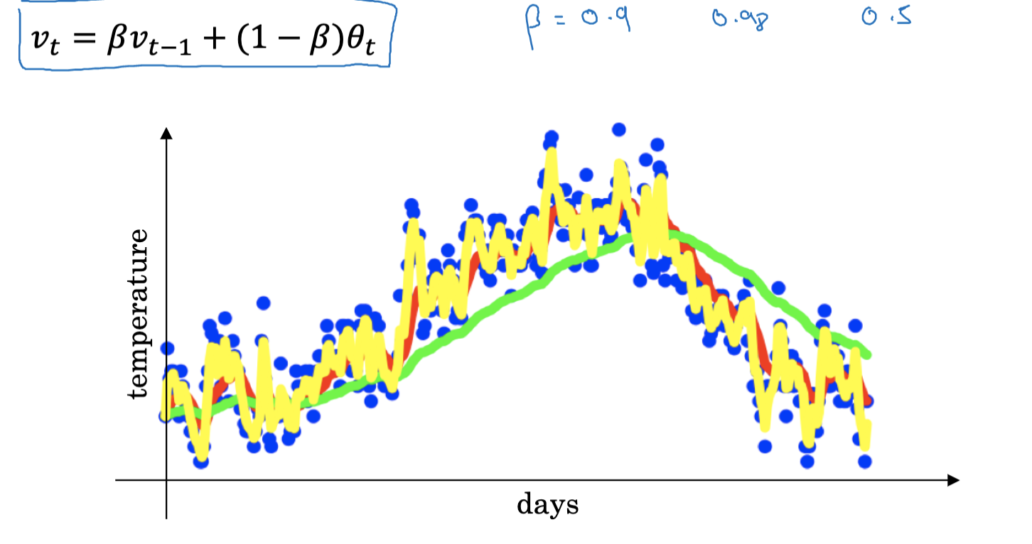
So, how many days of data does the Exponentially Weighted Average actually cover? If $\beta=0.9$, then the 10th power of 0.9 is about 0.35, meaning the weight decays to about 1/3 of its original value after 10 days. Therefore, when $\beta=0.9$, this formula essentially calculates the weighted average of the data from the past 10 days. Conversely, if $\beta=0.98$, it takes 50 days for the weight to decay to about 1/3 of its original value. Thus, we can view this formula as calculating the weighted average of the data from the past 50 days. Generally, we can think of this formula as averaging data over approximately $1/(1-\beta)$ days.

When implementing Exponentially Weighted Average, we need to initialize a value $V_0$ and then use the above formula to update $V_t$ for each time step $t$. During this process, it is not necessary to save all observations $x_i$, but only the latest $V_t$. The advantage of this method is that it occupies very little memory, needing only to retain one real number. While this is not the most accurate method of averaging, if you need the most accurate average, you should calculate the average of all values in a sliding window. However, this requires more memory and is more complex. In many situations where calculating the average of many variables is necessary, such as in deep learning, using Exponentially Weighted Average is both efficient and memory-saving.

Causes of Bias and Bias Correction

However, Exponentially Weighted Average has a minor issue: in the initial stages, due to the initialization of $V_0$ and the nature of weighted averaging, there can be some bias. Specifically, when we start calculating the average, it tends to be biased towards the initial value $V_0$ rather than the true average. One way to address this problem is through bias correction.
$$
\hat{V}_t = \frac{V_t}{1-\beta^t}
$$
In this formula, $\hat{V}_t$ is the corrected average, and $t$ is the time step. When $t$ is small, $\beta^t$ will be close to 1, making the correction term $1 - \beta^t$ small, resulting in a larger corrected average $\hat{V}_t$ and thus reducing the initial bias. As $t$ increases, $\beta^t$ approaches 0, making the correction term $1 - \beta^t$ approach 1, and the corrected average $\hat{V}_t$ approaches the uncorrected average $V_t$.

4. Momentum Gradient Descent

A common issue with the gradient descent algorithm is its inefficiency when the loss function is unbalanced, meaning it's much steeper in one direction compared to another. Momentum gradient descent addresses this by introducing the concept of "momentum."

Basic Idea

The concept of momentum gradient descent is inspired by physics, where an object's downhill velocity depends not only on the current slope (i.e., gradient) but also on its previous velocity (i.e., momentum). In optimization, past gradients act like velocity, and their exponentially weighted average represents momentum.

When optimizing a cost function with an elliptical contour, standard gradient descent can cause significant oscillations along the vertical axis, slowing down the process. Using a large learning rate can result in the algorithm "jumping" across the elliptical contour, preventing convergence.

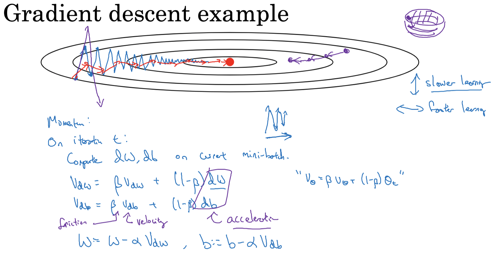
To address this, we use the momentum gradient descent method. In each iteration, we calculate the usual derivatives dw and db (using the current mini-batch or the entire dataset). We then compute the exponentially weighted averages of the gradients, vdw and vdb. The weights are updated using vdw and vdb instead of the original dw and db. This approach smooths the gradient descent steps, reducing vertical oscillations and speeding up horizontal movement.

Advantages

Momentum gradient descent's primary advantage is its ability to accelerate descent in flat directions while dampening oscillations in steep directions. In flat directions, smaller gradients mean past gradients dominate, speeding up movement. In steep directions, although current gradients are larger, the past gradients' positive and negative values average out, reducing movement in that direction.

5. RMSprop Optimization Algorithm

RMSProp (Root Mean Square Propagation) is an enhanced gradient descent algorithm that accelerates the optimization process by adjusting the learning rate dynamically. The core concept is that if a parameter has shown frequent changes in previous iterations, its learning rate should be decreased; conversely, if a parameter has shown infrequent changes, its learning rate should be increased. RMSprop was initially introduced in Geoffrey Hinton's Coursera course rather than in an academic paper.

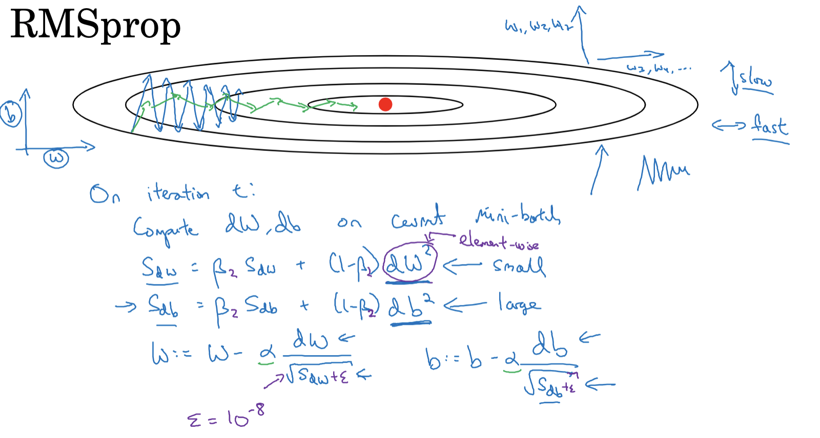
RMSprop Algorithm Steps

1. In each iteration ( t ), compute the gradients ( dW ) and ( db ) for the current mini-batch.
2. Calculate the exponentially weighted moving average of the squared gradients using the following formulas:
   • ( S{dW} = \beta S{dW} + (1-\beta) \cdot (dW)^2 )
   • ( S{db} = \beta S{db} + (1-\beta) \cdot (db)^2 )
     Here, ( \beta ) is a hyperparameter between 0 and 1, and the squaring operation is element-wise.
3. Update the parameters with the formulas:
   • ( W = W - \alpha \cdot \frac{dW}{\sqrt{S_{dW}} + \epsilon} )
   • ( b = b - \alpha \cdot \frac{db}{\sqrt{S_{db}} + \epsilon} )
     where ( \alpha ) is the learning rate, and ( \epsilon ) is a small constant to prevent division by zero, typically set to ( 10^{-8} ).

Analysis of RMSprop Working Principle

• RMSprop aims to provide different update speeds for different directions. For instance, in some dimensions (e.g., parameter ( b )), a slower learning rate is desired to reduce oscillations, while in other dimensions (e.g., parameter ( W )), a faster learning rate is preferred to accelerate convergence.
• To achieve this, RMSprop uses the squared gradient. If the gradient's absolute value in a certain direction (e.g., parameter ( b )) is large, its square will also be large, resulting in a higher ( S{db} ) value and thus a reduced update speed in that direction. Conversely, if the gradient's absolute value in a certain direction (e.g., parameter ( W )) is small, its square will be small, leading to a lower ( S{dW} ) value and thus an increased update speed in that direction.
• To prevent division by zero, a small constant ( \epsilon ) (typically ( 10^{-8} )) is added to the denominator.
• To differentiate from the momentum hyperparameter ( \beta ), the hyperparameter in RMSprop is often referred to as ( \beta_2 ).

Comparison with Momentum Gradient Descent

Compared to momentum gradient descent, RMSprop is more effective in dealing with varying gradient magnitudes in different directions. Momentum gradient descent primarily accelerates convergence by increasing the speed in directions with smaller gradient changes, whereas RMSprop adjusts the learning rate individually for each parameter, ensuring that all parameters are updated at an appropriate rate.

6. Adam Optimization Algorithm

Adam (Adaptive Moment Estimation) is an advanced gradient descent algorithm that integrates the concepts of both momentum gradient descent and RMSprop. The primary advantage of Adam is its ability to adaptively adjust the learning rate for each parameter, ensuring robust performance across various scenarios.

Basic Concept

Adam combines the benefits of momentum and RMSprop. The algorithm operates as follows:

1. Initialization: Set initial values $V{dw}=0$, $S{dw}=0$, $V{db}=0$, and $S{db}=0$.
2. Gradient Calculation: In each iteration ( t ), compute the gradients ( dw ) and ( db ), and update the exponentially weighted averages of the gradients:
   1. ( V_{dw} = \beta1 V{dw} + (1 - \beta_1) dw )
   2. ( V_{db} = \beta1 V{db} + (1 - \beta_1) db )
3. RMSprop-like Update: Update the exponentially weighted averages of the squared gradients:
   1. ( S_{dw} = \beta2 S{dw} + (1 - \beta_2) dw^2 )
   2. ( S_{db} = \beta2 S{db} + (1 - \beta_2) db^2 )
4. Bias Correction: Correct the bias for ( V ) and ( S ):
   1. ( V{dw}^{\text{corrected}} = \frac{V{dw}}{1 - \beta_1^t} )
   2. ( V{db}^{\text{corrected}} = \frac{V{db}}{1 - \beta_1^t} )
   3. ( S{dw}^{\text{corrected}} = \frac{S{dw}}{1 - \beta_2^t} )
   4. ( S{db}^{\text{corrected}} = \frac{S{db}}{1 - \beta_2^t} )
5. Parameter Update: Update the parameters:
   1. ( W = W - \alpha \frac{V{dw}^{\text{corrected}}}{\sqrt{S{dw}^{\text{corrected}}} + \epsilon} )
   2. ( b = b - \alpha \frac{V{db}^{\text{corrected}}}{\sqrt{S{db}^{\text{corrected}}} + \epsilon} )

The learning rate ( \alpha ) requires tuning, typically by experimenting with a range of values. The recommended default values are ( \beta_1 = 0.9 ), ( \beta_2 = 0.999 ), and ( \epsilon = 10^{-8} ). While ( \alpha ) is often adjusted during implementation, ( \beta_1 ) and ( \beta_2 ) adjustments are less common.

Adam stands for Adaptive Moment Estimation. ( \beta_1 ) is used to compute the mean of the gradient (first moment), while ( \beta_2 ) is used for the exponentially weighted average of the squared gradient (second moment).

This optimization algorithm merges the strengths of momentum and RMSprop, proving highly effective across a wide range of neural network architectures.

7. Learning Rate Decay

In many optimization algorithms, we need to set a learning rate parameter, which determines the magnitude of parameter updates. If the learning rate is too high, the optimization process might oscillate around the optimum and fail to converge; if the learning rate is too low, the optimization process might be extremely slow. Learning rate decay is a common technique that helps dynamically adjust the learning rate during training.

Concept

The basic concept of learning rate decay is to gradually decrease the learning rate as training progresses. This approach allows the use of a higher learning rate in the early stages when far from the optimum, facilitating rapid progress. As the process nears the optimum, a smaller learning rate is used for finer adjustments, reducing oscillations around the optimum.

Implementation Methods

There are several methods to implement learning rate decay, including the following:

• Time-based Decay: This common method reduces the learning rate linearly or exponentially over time. For example, we can set the learning rate as $\alpha / (1 + t / T)$, where $\alpha$ is the initial learning rate, $t$ is the current step number, and $T$ is a hyperparameter.

• Step Decay: In this method, the learning rate is reduced by a certain factor after a fixed number of steps. For example, the learning rate might be multiplied by 0.9 after every 1000 steps.

• Scheduled Decay: This method involves setting a predefined learning rate schedule and adjusting the learning rate according to this schedule. For instance, the learning rate might be set to 0.01 for the first 1000 steps, then reduced to 0.001 for the next 1000 steps, and so on.

8. The Problem of Local Optima

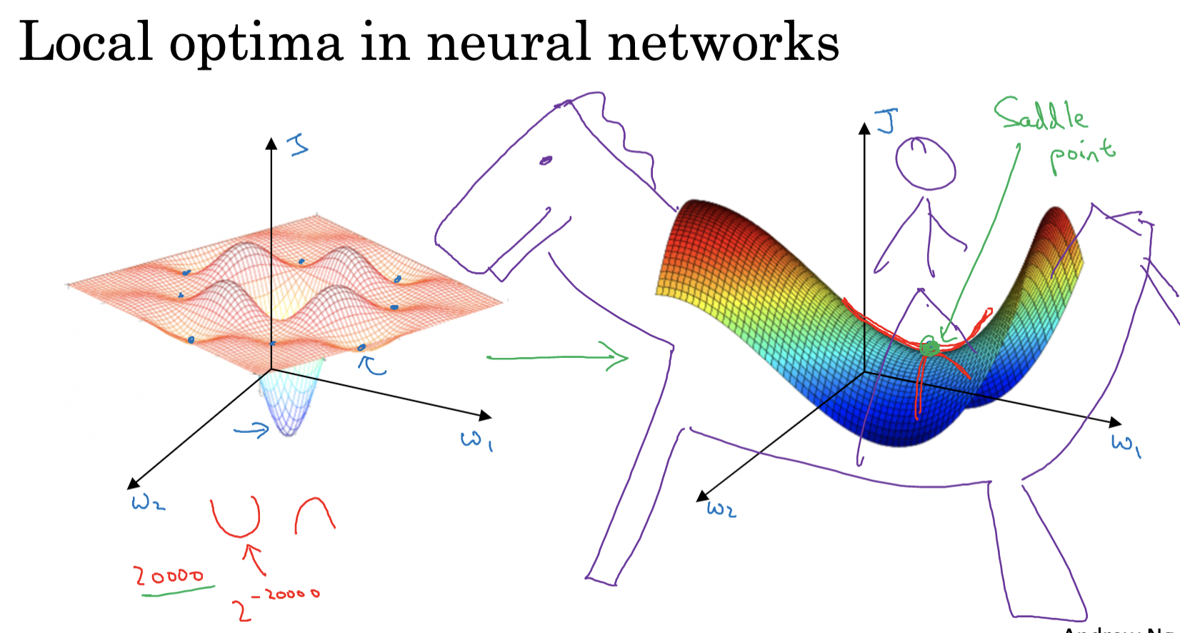
In the process of optimization, we often encounter the problem of local optima. A local optimum refers to the best point within a certain region of the parameter space, but it is not the best point in the entire parameter space (i.e., the global optimum). If our optimization algorithm gets stuck at a local optimum, we will not achieve the best model performance.

Local Optima and Deep Learning

However, in deep learning, even though local optima seem problematic, they are actually not as serious. This is because, in high-dimensional space, most local optima are actually "saddle points." At a saddle point, some directions are locally optimal, but in other directions, there may still be room for further optimization. Since deep learning models usually have a large number of parameters, even at a local optimum, there is a high probability of finding a direction that can be optimized, thus escaping the local optimum.

Moreover, many optimization algorithms, such as momentum gradient descent, RMSprop, and Adam, help us escape local optima. By accumulating past gradients, they help us search along directions of minor gradient changes, potentially finding a direction that can be optimized.

Randomness and Local Optima

Randomness also helps us escape local optima. In deep learning, since we often use mini-batch gradient descent, there is a certain randomness in each step's gradient. This means that even if we are at a local optimum, we may escape it due to the random gradients. Additionally, we can increase the randomness of the optimization process by adding noise or using random initialization methods, thereby having a greater chance of escaping local optima.

In this blog post, we have introduced various deep learning optimization techniques, including mini-batch gradient descent, exponential moving average, momentum gradient descent, RMSprop, Adam, learning rate decay, and the problem of local optima. We hope this knowledge helps you better train your models on your deep learning journey. Although there are many formulas in this chapter, it's okay if you don't remember them. In the subsequent development process, various machine learning frameworks will assist you, so you won't need to manually calculate these formulas. Thank you for reading, and see you in the next blog post!