Introduction to Convolutional Neural Networks

Convolutional Neural Networks (CNNs) are a type of deep neural network designed for image processing. Inspired by the structure of biological visual systems, CNNs utilize convolution operations to extract spatial features from images and combine these with fully connected layers for classification or prediction tasks. The integration of convolution operations allows CNNs to excel in image processing, making them widely applicable in tasks such as image classification, object detection, and semantic segmentation. This blog will provide a brief introduction to the basics of convolutional neural networks, based on the first week of Professor Andrew Ng's deep learning specialization, course four.

Starting with Computer Vision

Computer vision is a rapidly developing field within deep learning. It is used in various applications such as enabling autonomous vehicles to recognize surrounding vehicles and pedestrians, facial recognition, and displaying different types of images to users, like those of food, hotels, and landscapes. Convolutional neural networks are extensively used in image processing for tasks like image classification, object detection, and neural style transfer. Image classification involves identifying the content within an image, object detection identifies and locates objects in an image, and neural style transfer re-renders an image in a different style.

One challenge in computer vision is that the input images can be arbitrarily large. For instance, a 1000x1000 pixel image has an input feature dimension of 1000x1000x3, which entails processing a large amount of data. This can lead to overfitting and high demands on computation and memory. To address this issue, convolution operations are effectively utilized, which form the core of convolutional neural networks.

Edge Detection

Edge detection is a fundamental task in image processing that aims to identify areas in an image where pixel values change abruptly, marking the boundaries of objects. This can help in detecting shapes and contours of objects. Edge detection can be accomplished through convolution operations.

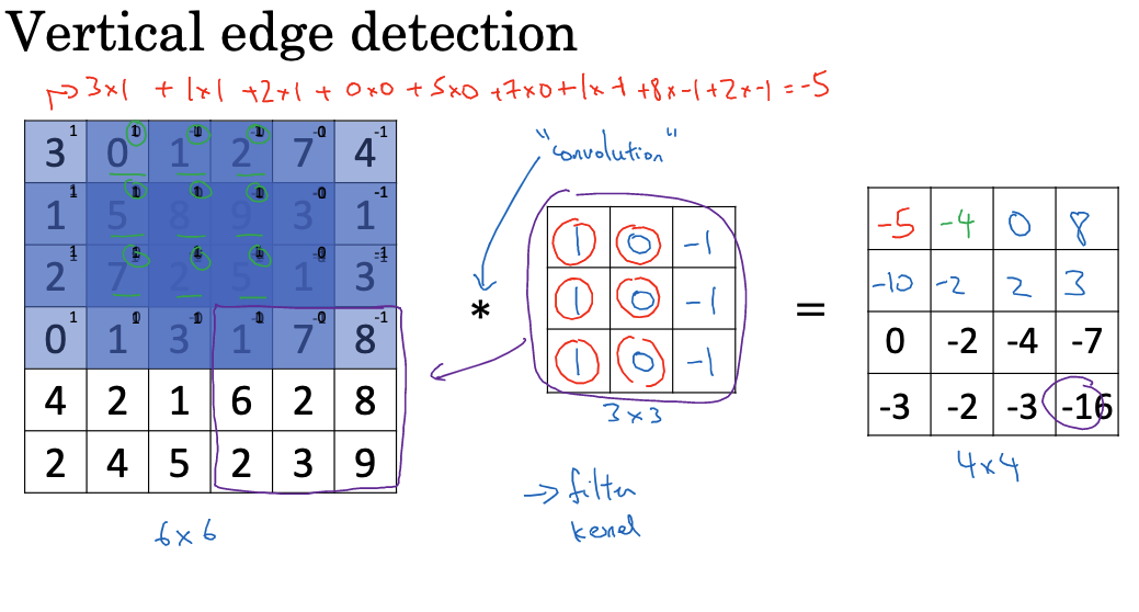
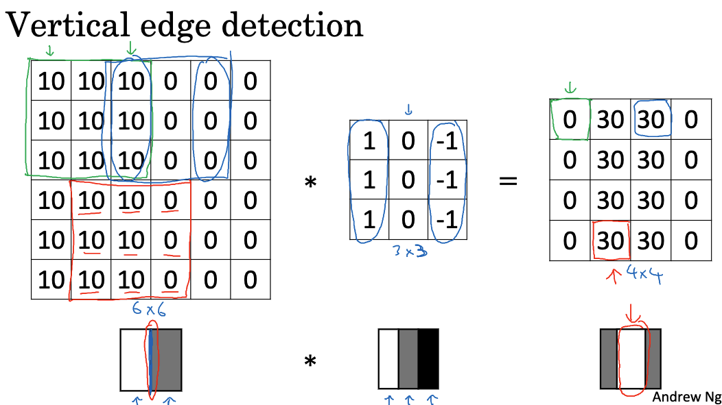
Suppose we have a 6x6 pixel grayscale image and we want to detect vertical edges. We can construct a 3x3 filter (also called a convolution kernel) with the following weight matrix:

1 0 -1
1 0 -1 
1 0 -1

This filter essentially performs a derivative operation to detect changes in the vertical direction. We slide this 3x3 filter over the image and compute the convolution at each position. For instance, at the top-left corner, the filter and the corresponding image region are element-wise multiplied and summed, resulting in an output value of -5. Repeating this process, we obtain a new 4x4 feature map.

Similarly, different filters can be used to detect horizontal edges, 45-degree edges, and more. This process of extracting basic image features using filters is the primary function of convolutional layers in CNNs. In practice, CNNs learn multiple sets of filters to detect edges in various directions simultaneously, yielding rich feature representations.

Different deep learning frameworks may implement convolution operations differently. For example, in TensorFlow, the tf.nn.conv2d function is used to perform convolution operations. Convolution operations help in detecting vertical edges by applying specific filters to the image. For example, if the left part of our image has a pixel value of 10 and the right part has a pixel value of 0, the convolution operation described above will reveal a bright vertical line, indicating the transition from the bright to the dark area in the original image.

Positive edges refer to transitions from bright to dark, while negative edges refer to transitions from dark to bright. Using different edge detectors allows us to distinguish various types of edges and enables the algorithm to automatically learn these detectors instead of setting them manually.

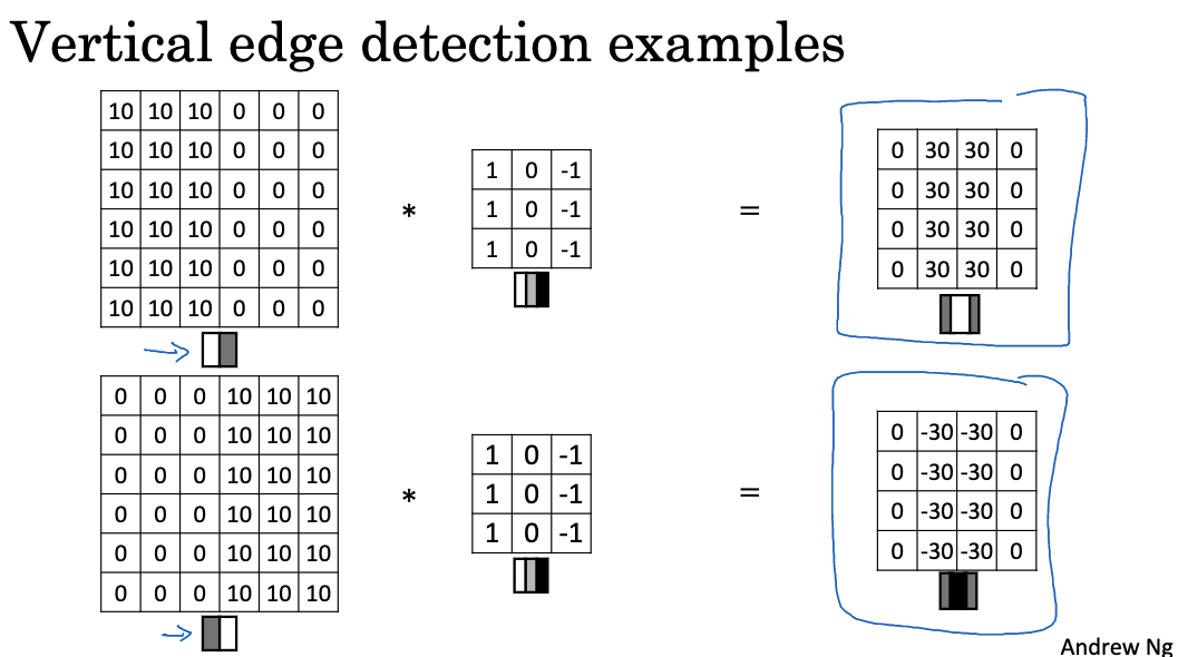
As illustrated above, convolving a 6x6 image with a vertical edge detector highlights the vertical edges in the middle part. If the colors are reversed, with the left side becoming dark and the right side becoming bright, the result will be the opposite, changing the original 30 to -30, indicating a dark-to-bright transition. By taking the absolute value of the output matrix, we can ignore the direction of the brightness change, but in practice, filters can distinguish between bright-to-dark and dark-to-bright boundaries.

Both vertical and horizontal edge detectors use 3x3 filters, though there is some debate about the optimal numerical combinations. Common choices include Sobel filters and Scharr filters, which differ in their weight distributions and performance characteristics.

Neural networks can learn the parameters of these filters through backpropagation to better capture the statistical features of the data. Neural networks can learn low-level features such as edges, which can be more stable than manually selected filters. Backpropagation can learn any required 3x3 filter and apply it to any part of the image to detect the desired features. By learning these 9 numbers as parameters, neural networks can automatically learn to detect vertical edges, horizontal edges, inclined edges, and other edge features.

Padding and Strided Convolutions

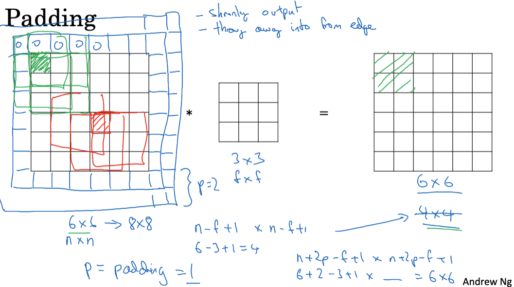
In convolution operations, padding is applied to ensure that the filter can cover the entire receptive field when it slides to the edge of the image. Common padding methods include zero padding and symmetric padding. Zero padding is the simplest method, where zeros are added to the image boundary. This ensures that the output feature map size is equal to the input image size minus the filter size plus one.

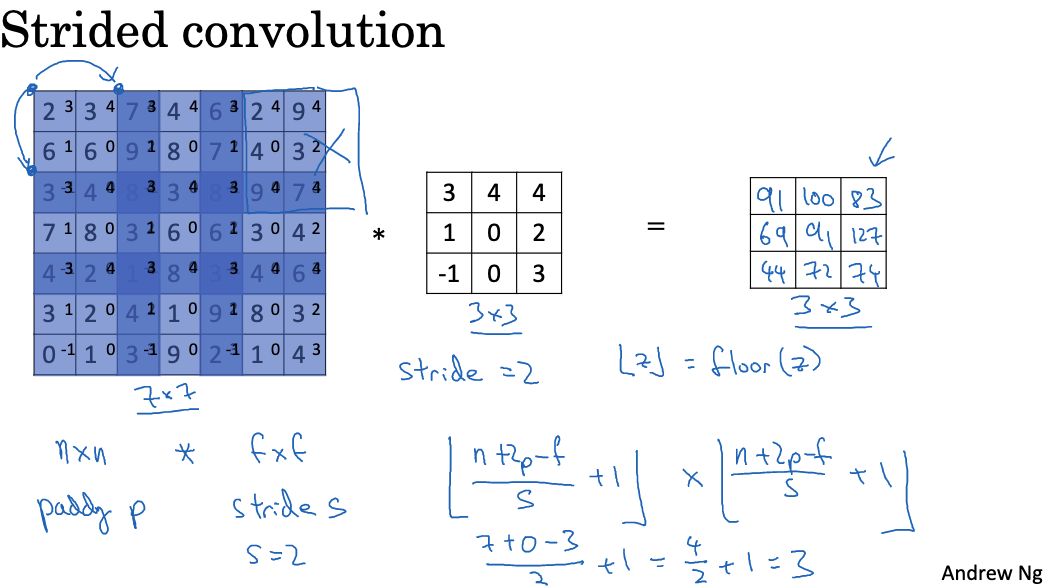
The stride parameter can also be used in the convolution layer to control the interval at which the filter slides, thereby reducing the size of the output feature map.

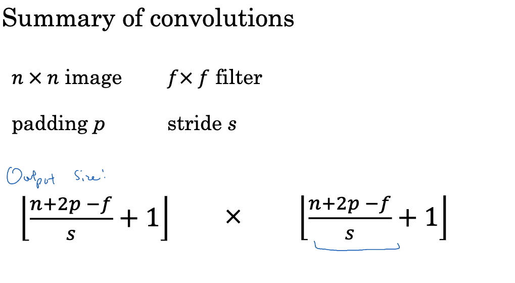
For example, using a 3x3 filter on a 7x7 image with a stride of 1 results in a 5x5 output feature map. However, if the stride is set to 2, the filter jumps one position at a time, resulting in a 3x3 output feature map. Generally, if the input size is n x n, the filter size is f x f, with padding p and stride s, then the output feature map size can be calculated as:
$$
\frac{n + 2p - f}{s} + 1
$$
The stride setting significantly affects the output feature map size. When the stride is greater than 1, the output feature map shrinks as the filter skips positions, which reduces the computational load in subsequent layers. This is often used in deeper network layers for dimensionality reduction. However, if the stride is set too large, it can lead to information loss. Especially in shallow networks, we typically want to extract all features of the input image, so the stride of the first convolution layer is usually set to 1.

When designing the network, we can control the scaling ratio of feature maps in intermediate layers by adjusting the stride and padding. A common setup is to use a convolution layer with a stride of 2 and padding of 1 to counteract the size reduction caused by pooling. Note that the zeros added during padding can affect feature extraction to some extent. Therefore, the number of padding layers should not be excessive, usually set to 0 or 1.

Additionally, besides stride and padding, the number of filters can be adjusted to change the number of output channels, and different filter sizes can be used to detect features of various scales. By combining these techniques, precise control over the output feature map of the convolutional layer can be achieved.
Note that during convolution operations, the filter must be entirely within the image or the padding area. If the filter exceeds the image range, that part of the calculation will not be performed. In some mathematical and signal processing literature, convolution operations require flipping the filter horizontally and vertically before performing element-wise multiplication and summation. However, in deep learning, we typically do not perform this flipping operation. In fact, what we call convolution is technically "cross-correlation," but in deep learning, we still refer to it as convolution.

3D Convolution

For RGB images, convolution operations need to be performed in three dimensions: width, height, and color channels. This requires the use of 3D filters.

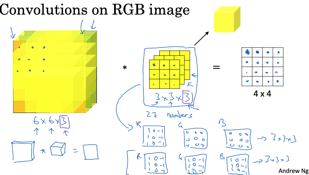
For example, for a 6 x 6 x 3 RGB image, we can define a 3 x 3 x 3 3D filter. This filter also has three color channels: R, G, and B. In the convolution operation, each value in the filter is multiplied by the corresponding pixel position and color channel value in the image. The sum of all these products gives one pixel value in the output feature map. Repeating this process yields a 4 x 4 2D output feature map. Each pixel in this map contains information from the three color channels at that position in the original image. The use of 3D filters allows convolution operations to extract features in both spatial and color dimensions. For example, one filter might be sensitive to green edges, while another might detect edges of all colors. 3D convolution kernels enable learning rich color features.

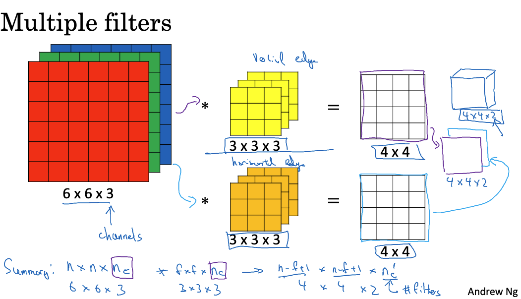
If we want to detect more features (such as vertical and horizontal edges), we can apply multiple filters simultaneously. Each filter generates one output image, and all output images can be stacked together to form a higher-dimensional output. For example, if we use two 3x3x3 filters to convolve a 6x6x3 image, we get two 4x4 outputs, which can be combined into a 4x4x2 output cube.

Each layer in a convolutional neural network can be seen as performing convolution operations. Different filters represent different neurons in the network, each dedicated to detecting a specific feature. This method of convolving over cubes can process RGB images and detect any number of features, enabling the neural network to handle more complex problems.

Single-layer Convolutional Network

Having understood how convolution operations work, let's look at how to build a single-layer convolutional neural network.

The workflow of a convolutional layer can be summarized in four steps:

Applying Filters: In a convolutional neural network, we first apply filters to the input through convolution. This involves point-wise multiplication of the input and summing the results to get a new value. This process is repeated for each filter, so if we have two filters, we get two separate results.
Adding Bias: Next, we add a bias to the result of each filter. This bias is a real number added uniformly to all elements.
Non-linear Transformation: Then, we apply a non-linear transformation to the bias-added results, such as the ReLU activation function.
Combining Results: Finally, we combine all the processed results to obtain a new multi-dimensional output. For example, if we used two filters, we get a new 4x4x2 output.

Throughout this process, each filter acts like a weight matrix in a neural network, performing linear transformations on the input. By adding bias and applying non-linear transformations, we get results similar to those produced by activation functions in neural networks.

Additionally, let's calculate the number of parameters in a single-layer convolutional neural network. This depends on the number and size of filters. For instance, a 3x3x3 filter has 27 parameters (corresponding to its volume), plus one bias, totaling 28 parameters. If there are 10 such filters in the network, there are 280 parameters in total.

Below is a summary of some symbols used in CNNs. Please take note.

An important feature of convolutional neural networks is parameter sharing. This means that the number of network parameters remains fixed regardless of the input image size. This helps reduce the risk of overfitting, as the number of parameters is small compared to the image size.

Simple Convolutional Network Example

Let's look at an example of a deep convolutional neural network used for tasks such as image classification and image recognition.

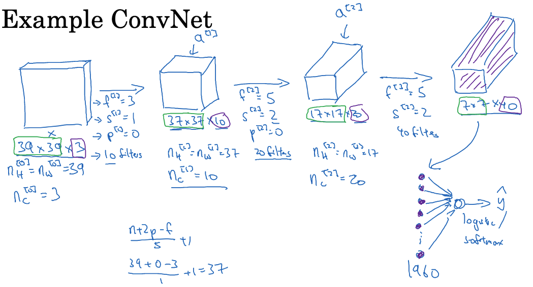
The network's input is a 39 x 39 x 3 image, with the goal of determining if the image contains a cat.
The network structure:
- First layer: Use 10 3x3 filters (no padding, stride 1) for convolution, output size is 37 x 37 x 10.
- Second layer: Use 20 5x5 filters (no padding, stride 2) for convolution, output size is 17 x 17 x 20.
- Third layer: Use 40 5x5 filters (no padding, stride 2) for convolution, output size is 7 x 7 x 40.
Finally, the obtained 7 x 7 x 40 feature map is flattened into a vector of 1960 units, which is then input to a logistic regression or softmax unit for classification.

When designing convolutional neural networks, the hyperparameters to choose include the number of units, stride, padding, and the number of filters. As the network depth increases, the height and width of the image usually decrease gradually, while the number of channels gradually increases. In a typical convolutional neural network, besides convolutional layers (Conv), pooling layers (Pool) and fully connected layers (FC) are often used. These two layers are simpler than convolutional layers.

Pooling Layer

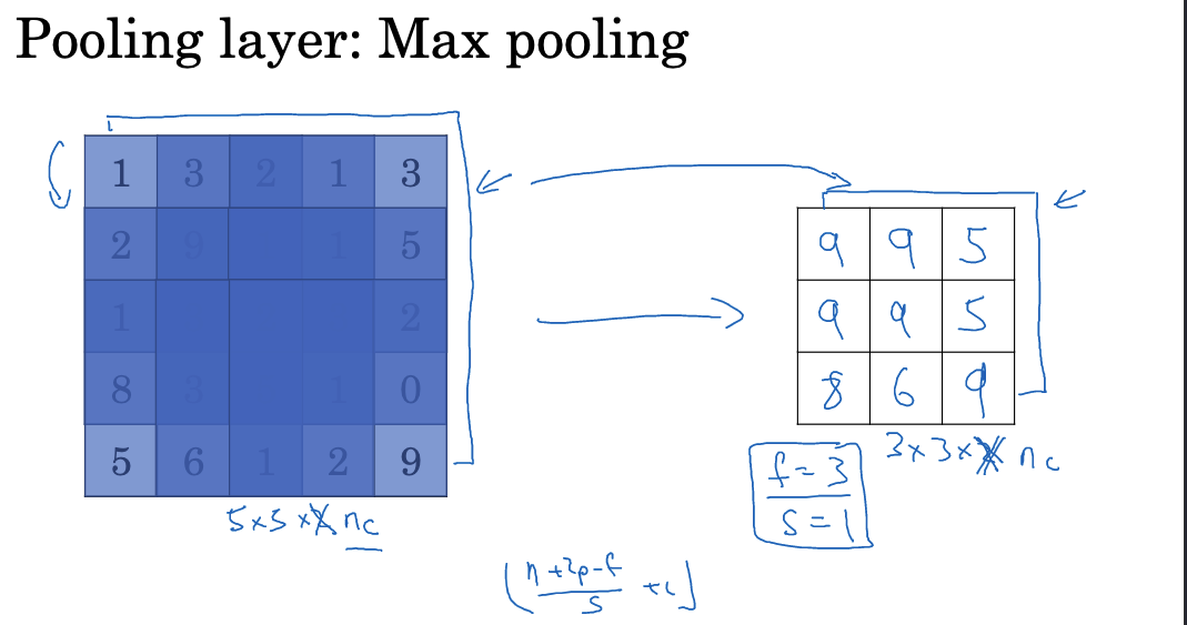
Besides convolutional layers, ConvNets often use pooling layers to reduce the size of feature maps. Pooling layers play a crucial role in convolutional neural networks. Their purpose is to reduce the dimensions of representations, increase computation speed, and enhance the ability to detect certain features. Common pooling methods include max pooling and average pooling.

For example, using a 2x2 max pooling with stride 2 on a 4x4 feature map results in a 2x2 output feature map. Each element in the output is the maximum element from the corresponding 2x2 region. The max pooling mechanism selects the maximum value from each region as the output. If a specific feature is detected anywhere in the filter region, the maximum value retains that feature. If the feature is not detected, the maximum value in that region is usually small. Thus, max pooling effectively detects features by selecting the maximum value and retaining these features in the output.

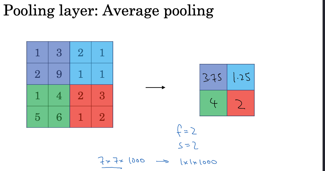
Average pooling is another sampling method, which takes the average value in each region. As shown below:

Max pooling is strong in extracting main features but may lose details in the feature map. Therefore, the strength of the pooling operation needs to be balanced in the design. Besides reducing feature map size, pooling layers do not contain any learnable parameters. This further optimizes the network structure and reduces the risk of overfitting. It is important to note that pooling layers can disrupt spatial relationships in feature maps. Overuse can lead to the loss of spatial information, so pooling is typically done in intermediate layers of the network. Additionally, the size of the pooling kernel needs to be chosen carefully. Too small a kernel limits feature extraction, while too large a kernel results in the loss of details.

Hyperparameters for the pooling layer include filter size (f) and stride (s). Common hyperparameter choices are f=2 and s=2, which reduce the height and width of the representation by more than half. Another common choice is f=2 and s=2, which halves the height and width of the representation.

A Complete Convolutional Neural Network Example

Let's examine a complete example of a convolutional neural network that utilizes convolutional layers, pooling layers, and fully connected layers:

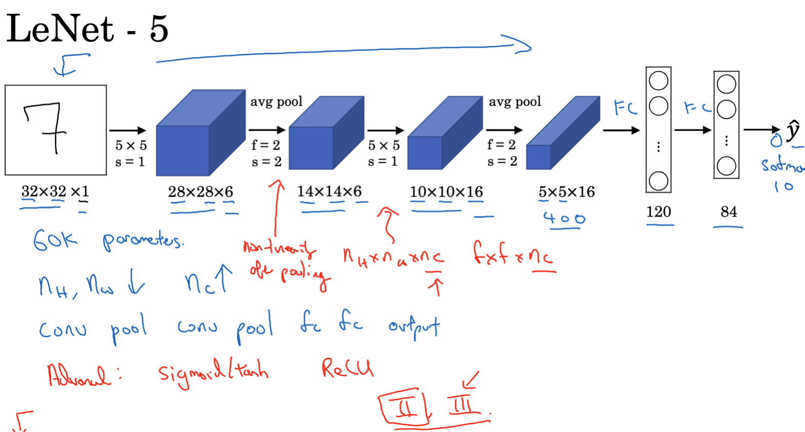
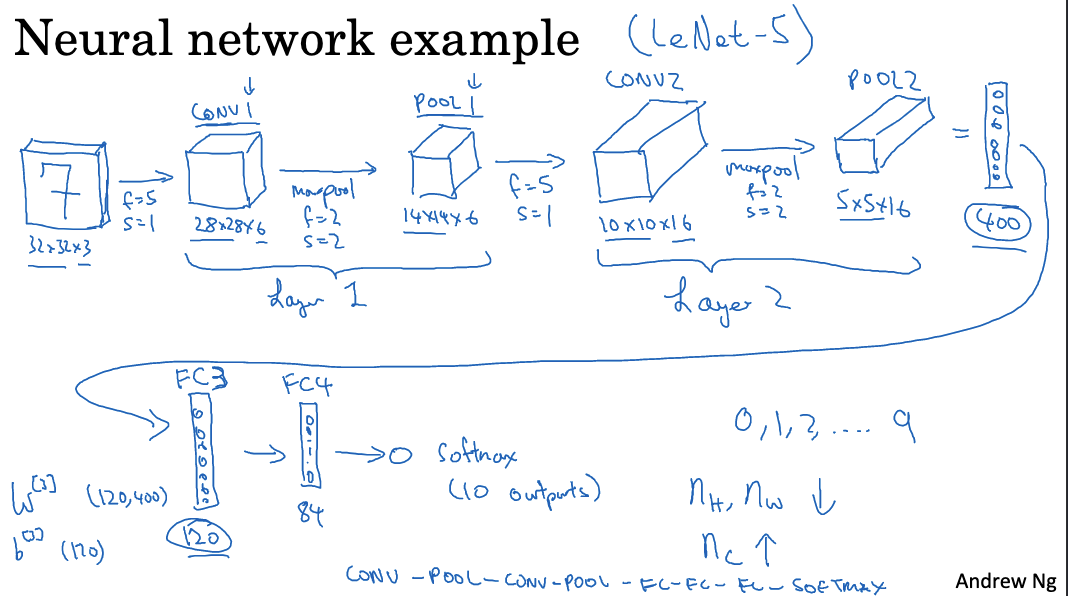
This example is inspired by the LeNet-5 architecture, though it is not identical.
The input image size is 32x32x3 (RGB image).
The first layer is Convolutional Layer 1, which uses 5x5 filters, a stride of 1, and 6 filters, resulting in an output size of 28x28x6.
Next, Pooling Layer 1 employs 2x2 max pooling with a stride of 2, producing an output size of 14x14x6.
Convolutional Layer 2 follows, using 5x5 filters, a stride of 1, and 10 filters, with an output size of 10x10x10.
This is followed by Pooling Layer 2, which uses 2x2 max pooling with a stride of 2, yielding an output size of 5x5x10.
Then, Convolutional Layer 3 uses 5x5 filters, a stride of 1, and 16 filters, resulting in an output size of 1x1x400.
The output from Pooling Layer 2 is flattened into a 400x1 vector.
Next is Fully Connected Layer 4, which has 120 units.
The final layer is Fully Connected Layer 5, with 84 units.
The final output layer is a Softmax layer with 10 units, used for the handwritten digit recognition task.

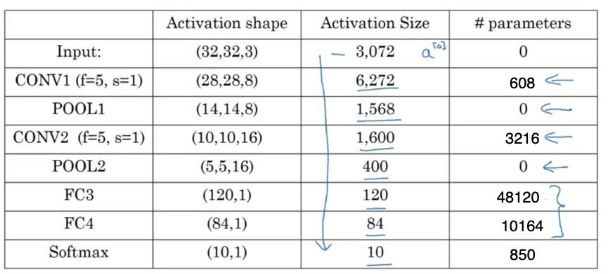
Details about the network include:

The input activation size is 32x32x3, corresponding to 3072 activation inputs.
The sizes and dimensions of the activation inputs for each layer are shown in the table.
Convolutional layers have relatively few parameters, while fully connected layers have more.
As the network deepens, the activation input size gradually decreases while the number of channels increases.
A typical network model alternates between convolutional and pooling layers, ending with fully connected layers and a Softmax layer.
The number of layers in a neural network usually refers to the layers with weights and parameters, with pooling layers typically not counted.

Suggestions for choosing hyperparameters:

Do not try to create your own set of hyperparameters; instead, refer to the literature to understand the hyperparameter combinations used by others.
Choose hyperparameter combinations that have worked for others, as they are likely to work for your application as well.
As the network deepens, it is common to decrease the height and width while increasing the number of channels.
When choosing hyperparameters, refer to common parameter combinations, such as using pooling layers with f=2 and s=2.

The design of convolutional networks needs to consider feature extraction, classification judgment, and optimization constraints. With the continuous development of various model designs, convolutional neural networks have performed excellently in computer vision and image processing. It is worth exploring their design principles.

Advantages of Convolutional Layers

Compared to fully connected layers, convolutional layers have two significant advantages:

Parameter Sharing:
In the same convolutional layer, all receptive fields use the same filter weight matrix. This means a filter uses shared parameters as it slides across the entire input image, greatly reducing the number of parameters.

For example, if the input image is 1000x1000x3 and we use 100 10x10x3 filters, without parameter sharing, there would be 300,000 parameters (100x10x10x3). With parameter sharing, there are only 30,000 parameters, reducing the number by an order of magnitude.

Parameter sharing not only reduces storage space but also significantly reduces the burden of model optimization. Only one set of filter weights needs to be updated per iteration.
Sparse Connectivity:
Sparse connectivity means that each output value is only related to a small part of the input, reducing the number of connections.

In a convolutional layer, each neuron is only connected to a local area of the input, not fully connected. For example, in a 10x10 filter, each neuron is only connected to 100 inputs, significantly reducing the number of parameters. This sparse connectivity ensures that the learned parameters can better detect local features and extract spatial information from the input.
Sparse connectivity also alleviates overfitting. Each neuron in the convolutional layer only responds to local features, which are combined to form overall features, making it less prone to high variance.

Convolutional neural networks can capture translational invariance, meaning that for a translated image, they can produce similar features and give the same label.

The steps to train a convolutional neural network include randomly initializing the parameters, calculating the cost function, and then using gradient descent or other optimization algorithms to optimize the parameters to reduce the cost function value.

In practice, you can refer to convolutional neural network structures published in research papers and use them in your applications.

Summary

Through the introduction of these concepts, I believe you have gained a preliminary understanding of the working principles and components of convolutional neural networks. Convolutional layers significantly reduce the number of parameters while preserving the spatial information of the image, which is key to the success of CNNs in handling image tasks.

Additionally, convolutional neural networks have some limitations, such as poor applicability to non-grid data and less convenient inter-layer connections compared to fully connected layers. Therefore, using CNNs requires considering the intrinsic characteristics of the problem and appropriately combining them with other network structures to maximize their effectiveness.

Convolutional neural networks have been widely used in computer vision and image processing, but their design and optimization still require continuous research and innovation. We look forward to seeing further development in CNN structure design, enabling better solutions to practical complex problems.