The primary focus of this blog is on hyperparameter tuning, batch normalization, and common deep learning frameworks. This is also the final week of the second course in the specialized deep learning curriculum. Let's dive in!

Hyperparameter Tuning

Hyperparameter tuning is a crucial process in deep learning. Properly setting hyperparameters will directly impact the performance of deep learning models. This section will explore the significance of hyperparameter tuning, the key hyperparameters that affect model performance, and methods and strategies for selecting these hyperparameters.

The Importance of Hyperparameter Tuning

Hyperparameter tuning has a decisive effect on the performance of deep learning models. Properly set hyperparameters can significantly enhance model training efficiency, generalization ability, and testing results. Conversely, improper hyperparameter choices can lead to slow training, ineffective learning, overfitting, and other problems.

The importance of hyperparameter tuning is reflected in the following aspects:

1. Hyperparameters directly influence the model's complexity, thus affecting its learning capability. A model with appropriate complexity can fully learn the data patterns while avoiding overfitting.
2. Different hyperparameters can affect the speed of model training. Choosing the right batch sizes, learning rates, and other settings can greatly accelerate model training.
3. Hyperparameter settings influence model convergence. Proper hyperparameters can help the model achieve faster and more stable convergence.
4. Hyperparameter selection is closely tied to regularization techniques, which directly affect the model's generalization ability.
5. Hyperparameters impact the model's optimization process. Different hyperparameter combinations lead to entirely different dynamics in the loss function during training.
6. In deep learning, deriving optimal hyperparameter settings theoretically is often challenging; it usually relies on experience and experimental results. Therefore, hyperparameter tuning is more of an experimental process.

In summary, hyperparameter tuning is a critical experimental process in deep learning, directly influencing the model's final performance. Hence, continuous experimentation is necessary to find the optimal hyperparameter combination, which requires substantial time and computational resources. However, the benefits of hyperparameter tuning are considerable, as it can greatly improve the effectiveness of deep learning models.

Key Hyperparameters Affecting Model Performance

Deep learning models contain numerous hyperparameters, but not all of them significantly impact model performance. The key hyperparameters that primarily affect model performance include:

1. Learning Rate
The learning rate is one of the most important hyperparameters in deep learning model training. It determines the step size of the Gradient Descent optimization algorithm in the parameter space. A learning rate that is too small will result in slow or stalled training, while a learning rate that is too large will lead to unstable training dynamics. The learning rate needs to be set within a reasonable range, typically found through experimentation.

2. Batch Size
The batch size determines the number of samples processed during each forward and backward propagation. A smaller batch size introduces more noise but allows for more frequent parameter updates; a larger batch size results in lower variance in gradient estimates for each batch, stabilizing training but requiring more computational resources and time. Generally, setting the batch size to 16, 32, 64, 128, etc., is reasonable for most models.

3. Weight Initialization Method
Different weight initialization methods affect the training speed and effectiveness of deep learning models. Common initialization methods include random initialization, Xavier initialization, etc. Proper initialization can accelerate model convergence and help avoid gradient vanishing or exploding issues.

4. Choice of Optimizer
Common optimizers in deep learning include SGD, Momentum, RMSProp, Adam, etc. Different optimizers result in significantly different dynamics of the loss function during training. Generally, SGD is suitable for simple models, while adaptive learning rate optimizers like Adam are more effective for complex deep models.

5. Regularization Strength
Regularization techniques (L1 regularization, L2 regularization, Dropout, etc.) are used to suppress overfitting and prevent the model from becoming too complex. The strength of regularization determines the extent of this suppression. Too little regularization leads to overfitting, while too much leads to underfitting. Multiple experiments are usually required to find the optimal regularization strength.

6. Network Depth and Width
Network width refers to the number of hidden units per layer, and network depth refers to the number of layers in the model. These two hyperparameters jointly determine the network's representational capacity and complexity. Setting an appropriate network width and depth can accommodate data patterns and prevent underfitting.

7. Learning Rate Decay Strategy
Learning rate decay involves gradually reducing the learning rate as training iterations increase. Common learning rate decay strategies include step decay, exponential decay, etc. An appropriate decay strategy can accelerate model convergence and improve testing results.

These seven hyperparameters can be considered the key factors influencing the performance of deep learning models. However, in practice, the importance of some other hyperparameters may vary depending on the specific model structure and dataset. Therefore, it is necessary to focus on the most influential hyperparameters for the target model and dataset when tuning.

How to Choose Hyperparameter Values

Choosing hyperparameters typically relies on both experimentation and experience. Here are some common strategies:

1. Grid Search: This method involves setting a range of values for each hyperparameter and then trying every possible combination. While it can identify the best hyperparameter set, it is computationally expensive, particularly when there are many hyperparameters to tune.
2. Random Search: Instead of trying every combination, this method randomly selects values within the defined range for each hyperparameter. This approach is less computationally intensive and can often explore the hyperparameter space more effectively, making it more likely to find good settings when there are many hyperparameters.

Once a promising hyperparameter set is found, a finer search can be conducted around it, known as local search. This involves setting smaller ranges for each hyperparameter and using grid or random search within these limits. This targeted approach helps find better hyperparameter settings with fewer trials.

Using appropriate scales for hyperparameters is crucial. For instance, learning rates typically range from 0.0001 to 1, but uniform sampling within this range is not ideal. Since the impact of learning rates on model performance follows a logarithmic scale, it’s better to select them logarithmically. Typically, an initial learning rate is chosen, and in each iteration, it is multiplied by a factor less than 1 (e.g., 0.9 or 0.99). This allows the model to learn quickly at first and fine-tune more precisely later.

Hyperparameter Tuning in Practice

Hyperparameter choices significantly affect deep learning outcomes. These choices may vary by field, but common strategies can often be applied across different domains. Hyperparameter settings that work well in one area might be effective in another, a strategy known as cross-domain transfer.

In practice, a set of optimal hyperparameters might need adjustments due to changes in datasets or hardware. Regular re-evaluation of hyperparameters, at least every few months, is recommended to maintain optimal performance.

There are two practical approaches to hyperparameter tuning:

• Panda Mode: This approach involves closely monitoring and adjusting a single model, ideal for scenarios with limited resources. It requires careful attention to the learning curve and continuous hyperparameter adjustments to optimize performance.
• Caviar Mode: Suitable for resource-rich environments, this approach involves training many models in parallel with different hyperparameter settings, then selecting the best performing set.
  
  
  
  Choosing between panda mode and caviar mode depends on your computational resources. With sufficient resources, caviar mode allows extensive experimentation with various hyperparameters. However, in fields like online advertising or computer vision, where massive data and numerous models are common, panda mode might be more appropriate.

While some hyperparameter settings can be generalized across tasks, others are task-specific. Balancing generality and specificity requires practical experience and careful consideration of the problem at hand.

Batch Normalization

Batch normalization is a crucial technique in deep learning, designed to accelerate network training and enhance model generalization. This section provides a comprehensive overview of the mechanism, effects, and practical considerations of batch normalization.

The Working Principle of Batch Normalization

To understand batch normalization in depth, we derive its process through detailed mathematical principles:

Assume there are m samples in a mini-batch, and the output of a certain layer in the network is $x_1, x_2, ..., x_m$. First, we calculate the mean and variance of this batch:

$$
\mu = \frac{1}{m} \sum_{i=1}^{m} xi
$$
$$
\sigma^2 = \frac{1}{m} \sum{i=1}^{m} (x_i - \mu)^2
$$

Using these statistics, we normalize the data:
$$
\hat{x}_i = \frac{x_i - \mu}{\sqrt{\sigma^2 + \epsilon}}
$$

Here, $\epsilon$ is a small constant added for numerical stability.

At this point, the data is normalized to have a mean of 0 and a variance of 1. However, this changes the original data's representation range. Therefore, we apply an inverse transformation to restore the data's representational capacity:
$$
y_i = \gamma \hat{x}_i + \beta
$$
Here, $\gamma$ and $\beta$ are learnable parameters that restore the original mean and variance of the data. This ensures that the normalized data retains its expressive power.

The above method is used during training. During the testing phase, batch statistics are not available. Hence, we use the moving average method, estimating the mean and variance with their exponential moving averages computed during training.

Why Batch Normalization is Effective

Batch normalization (BN) is effective in deep neural networks for several reasons:

1. It reduces the model's sensitivity to initial parameter values. Initializing network weights correctly is crucial, but finding the optimal values through random initialization is challenging. By normalizing inputs, BN makes the network less dependent on the initial parameter values.
2. It provides a regularization effect. The randomness introduced by batch statistics is similar to the effect of dropout, helping to mitigate overfitting slightly.
3. It accelerates network training. Normalization ensures consistent distribution across layers, allowing each training batch to be trained with a larger learning rate.
4. BN helps to alleviate gradient vanishing issues. By normalizing each layer's input values to a reasonable range, gradients are maintained more effectively.
5. Finally, BN allows for smaller weight decay to prevent overfitting, further enhancing performance.

In summary, batch normalization's strength lies in its ability to speed up training, improve generalization, reduce gradient vanishing, and provide regularization. These combined effects make it a crucial technique for enhancing deep neural network performance.

Batch Normalization in the Testing Phase

During training, a batch of data is used to calculate mean and variance. However, during testing, we typically process one sample at a time, making it impossible to calculate these statistics. To address this, we retain running mean and variance during training, using these running statistics for normalization during testing.

Specifically, we use the exponential moving average method to calculate the running mean and variance:

$$
\mu{running} = \alpha \mu{running} + (1-\alpha)\mu{batch}
$$
$$
\sigma^2{running} = \alpha \sigma^2{running} + (1-\alpha)\sigma^2{batch}
$$

Here, α is a decimal close to 1 (e.g., 0.9 or 0.99), while $\mu{batch}$ and $\sigma^2{batch}$ are the current batch's mean and variance. This approach estimates the entire training data distribution, which is then used for normalization during testing.

Application Recommendations for Batch Normalization

For effective use of batch normalization, consider the following suggestions:

1. The BN layer is typically placed after fully connected or convolutional layers, before the activation function. Avoid placing the BN layer at the network's beginning or end. However, for non-saturating activation functions like ReLU, placing BN after the activation function is also acceptable, and both configurations are often viable in practice.
2. BN can be combined with other regularization methods like Dropout. BN normalizes input distribution, while Dropout introduces random perturbations. Both provide orthogonal regularization effects. Note that due to BN's normalization, Dropout may be less effective than in standard networks, requiring additional adjustments when used together.
3. For small datasets, batch statistics can be noisy. Use larger batch sizes or continuously integrated batch statistics.
4. Update BN parameters after updating network parameters. First, calculate necessary statistics, then update parameters.
5. Encapsulate the BN process as a function or module for convenient use at any network position.
6. For small batch sizes, reduce the learning rate accordingly, as BN's regularization effect will be weaker.

Multi-class Classification

For multi-class classification problems, we typically use the softmax regression model. This section will provide a detailed introduction to the concept, principles, implementation, and application techniques of softmax regression.

Overview of Softmax Regression

Softmax regression is a generalized form of logistic regression and can be viewed as a log-linear regression for multi-class problems. By incorporating the softmax function, it converts the network output values into probabilities for each class, thus achieving multi-class classification. Compared to the One-vs-All method, softmax regression does not require training multiple binary classifiers. It directly provides the probabilities for each class, making it more concise and efficient. Softmax regression has become one of the standard solutions for multi-class classification problems.

Principles of Softmax Regression

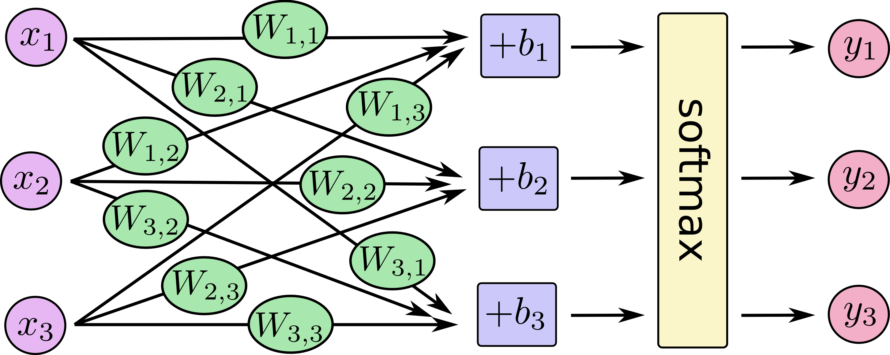
Assuming we have a dataset containing m samples, each sample x belongs to one of n classes. We define a linear model that outputs a vector z containing n elements for each sample, where each element represents the "score" of the corresponding class. Our goal is to train this linear model so that the score for the true class of sample x is the highest.

To achieve this, we first use the softmax function to normalize z into a probability distribution p:

$$
p_i = \frac{e^{zi}}{\sum{j=1}^n e^{z_j}}
$$

where ( p_i ) is the predicted probability that the sample belongs to the i-th class, and ( z_i ) is the original score given by the linear model.

We then use the cross-entropy loss function to measure the distance between the prediction and the true labels:

$$
J(\theta) = -\sum{i=1}^m \sum{j=1}^n y{ij} \log(p{ij})
$$

Here, if sample i belongs to class j, then ( y_{ij} = 1 ), otherwise it is 0.

Finally, by optimizing the loss function through the gradient descent algorithm, we can obtain a trained softmax regression model. For new samples, we calculate its score vector z, convert it to probabilities using softmax, and choose the class with the highest probability as the prediction result.

Implementation of Softmax Regression

Using Python and some machine learning libraries such as TensorFlow, we can easily implement softmax regression. The main steps include:

1. Constructing the computation graph with input features x and output score vector z. Here, z usually consists of two fully connected layers with nonlinear activation.
2. Applying the softmax function to z to obtain probability p. The softmax computation can be achieved using tf.nn.softmax().
3. Defining the cross-entropy loss function to automatically calculate the loss for all samples. This can be done using tf.nn.sparse_softmax_cross_entropy_with_logits().
4. Setting up the optimizer to iteratively train and update parameters to minimize the loss function. Common optimizers include SGD, Adam, etc.
5. After obtaining the trained model, to predict the class of new samples, first obtain z through the model, then convert to probability p using softmax, and choose the class with the highest probability.

Application Techniques of Softmax Regression

Softmax regression is a simple and effective multi-class classification model. The following techniques can help improve its performance:

1. For problems with a large number of categories, hierarchical softmax can be used, performing coarse classification first, then fine classification.
2. By increasing the loss weight of easily misclassified categories, the recognition effect of each category can be balanced.
3. Combining softmax regression with other scoring models for ensemble learning can achieve better classification performance.
4. By visualizing the classification decision boundary of the softmax model, the rationality of the classification can be intuitively judged and corresponding measures can be taken to improve the model.
5. The softmax model can pre-train semantic feature representations and then serve as the basis for downstream models, achieving transfer learning.
6. Adding a batch normalization layer to the last layer can avoid gradient instability and act as regularization.
7. The confidence of the prediction results is also useful; it can be used to filter low-confidence predictions or request manual review.

In summary, softmax regression is a simple yet effective multi-class classification model worth in-depth research and application to solve more practical problems.

Introduction to Deep Learning Frameworks

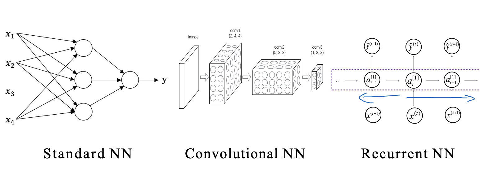
We can implement deep learning algorithms from scratch using Python and NumPy to understand how the algorithms work. However, implementing complex deep learning models, such as Convolutional Neural Networks (CNNs) and Recurrent Neural Networks (RNNs), can be very difficult. In fact, in the field of deep learning, there are many excellent open-source frameworks that provide tools for researchers and engineers to build, train, and deploy neural network models, such as TensorFlow and PyTorch.
So how to choose a deep learning framework? The following points are very important:

• Ease of programming: It is beneficial for the development and iterative improvement of neural networks and their deployment in a production environment.
• Running speed: When training on large datasets, some frameworks allow you to run and train neural networks more efficiently.
• True openness: A truly open-source framework needs not only open-source code but also good management. You should trust frameworks that will remain open source for the long term, not controlled by a single company.
  Of course, sometimes the choice of framework also depends on your programming language preferences and the type of application you are building. Choosing the right framework can make you more efficient in developing machine learning applications.

This is the end of this blog. I hope it will be helpful to you. Feel free to provide feedback.