In the rapidly evolving field of deep learning, innovative neural network architectures are constantly emerging. Keeping pace with these developments necessitates the study of these case studies. This blog is based on the content from the second week of the fourth course in Professor Andrew Ng's deep learning specialization, focusing on some case studies of convolutional neural networks.

Significance of Case Studies

Firstly, consider why we need to study these cases.

• These case studies embody the knowledge and experience accumulated by predecessors in network design. By studying these cases, we can intuitively understand successful design concepts and gain a deeper understanding of how to design network structures.
• Secondly, excellent network architectures often possess transferability. The structure of AlexNet, which solved the ImageNet classification problem, can also be applied to other visual tasks. Learning these architectures can help us design general models.
• Thirdly, reading papers is a way to improve oneself. Understanding the development of cutting-edge technologies helps broaden our horizons and enhances our analytical and learning abilities. Even if one is not engaged in visual research, these skills can be transferred to other fields.
• Finally, these cases come from top researchers, and their ideas are cutting-edge and unique. Studying these cases can not only help us build models but also broaden our thinking and stimulate our creativity.

Therefore, deeply understanding classic deep learning network cases will provide us with significant insights and help. Now, let's look at some of these important cases.

Classic Networks in Image Classification

In recent years, many epoch-making new models have emerged in the field of image classification, such as LeNet-5, AlexNet, and VGGNet.

LeNet-5 was proposed by Yann LeCun in 1998. It is an early convolutional neural network (CNN) structure used for digit recognition (especially handwritten digit recognition). This network model achieved very high recognition accuracy at the time and had a significant impact on subsequent convolutional neural network architectures. Here are some key components of LeNet-5:

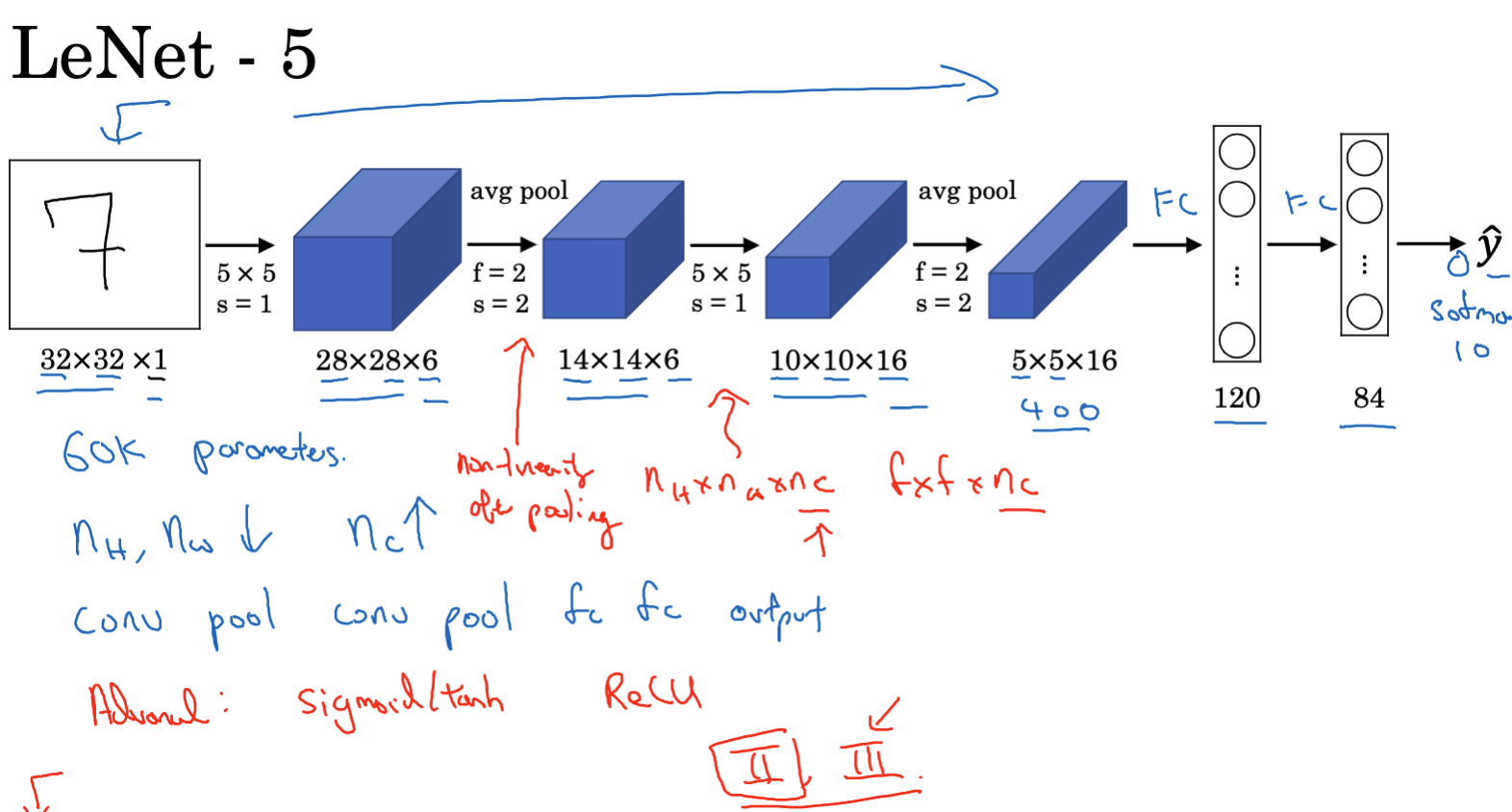
• Input layer: Receives a grayscale image of size 32x32x1. The '1' here refers to the number of channels, which is 1 for a grayscale image.
• First layer (convolution layer): Uses 6 convolution kernels of 5x5, stride 1, no zero padding. This outputs a feature map of 28x28x6.
• Second layer (pooling layer/subsampling layer): Uses a 2x2 filter for average pooling, stride 2. This reduces the image size to 14x14x6.
• Third layer (convolution layer): Uses 16 convolution kernels of 5x5, stride 1, no zero padding. The output size is 10x10x16.
• Fourth layer (pooling layer/subsampling layer): Uses a 2x2 filter for average pooling, stride 2. The output size is 5x5x16.
• Fully connected layer: After several convolutional and pooling layers, LeNet-5 uses several fully connected layers. First, the 5x5x16 output is flattened to 400 nodes, then connected to a fully connected layer with 120 nodes, followed by another fully connected layer with 84 nodes.
• Output layer: The final layer is a 10-node output layer corresponding to the handwritten digits 0-9.

LeNet-5 has the following characteristics:

• Average pooling: At that time, average pooling was more commonly used than the now more popular max pooling.
• Activation functions: Unlike modern networks, LeNet-5 used Sigmoid or Tanh activation functions more often than the now more commonly used ReLU.
• Number of parameters: The network is relatively small, with about 60,000 parameters.

LeNet-5 is a significant milestone in the history of convolutional neural networks because it was the first convolutional neural network successfully applied to digit recognition tasks. Although modern network structures are more complex and efficient, the basic design of LeNet-5 still influences many network architectures today.

AlexNet, proposed by Alex Krizhevsky et al. in 2012, achieved a historic breakthrough in the 1000-class image classification task at that time. Its structure mainly includes:

• The input image size is 227x227x3 (note that the paper mentions 224x224x3, but 227x227 may be more reasonable).
• The first layer uses 96 11x11 filters, stride 4, resulting in a 55x55 image.
• Next is a 3x3 max pooling layer, stride 2, reducing the volume to 27x27x96.
• Then a similar 5x5 convolution is performed, resulting in an output of 27x27x256.
• After max pooling, the height and width are both reduced to 13.
• By continuously performing 3x3 convolution operations, the result is finally reduced to 6x6x256.
• Flatten this result to obtain 9216 nodes, pass through several fully connected layers, and finally use softmax to output the result (one of the 1000 classes).
• The structure of AlexNet is similar to LeNet, but the number of parameters increased from 60,000 to about 60 million.

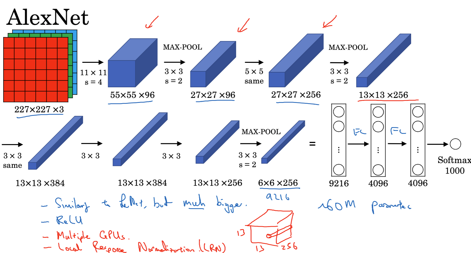
AlexNet demonstrated the powerful capabilities of large-scale deep convolutional neural networks and is considered a milestone in the field of deep learning.

Following closely is VGGNet, whose structure is simpler and focuses more on convolutional layers, making the structure uniform:

• All convolution filters are 3x3, stride 1, with the same padding.
• All max pooling layers have 2x2 filters, stride 2.
• The network contains 16 weight layers with a total of approximately 138 million parameters.
• The structure is concise and easy to understand. Despite the huge number of training parameters, its structural uniformity makes it widely used.

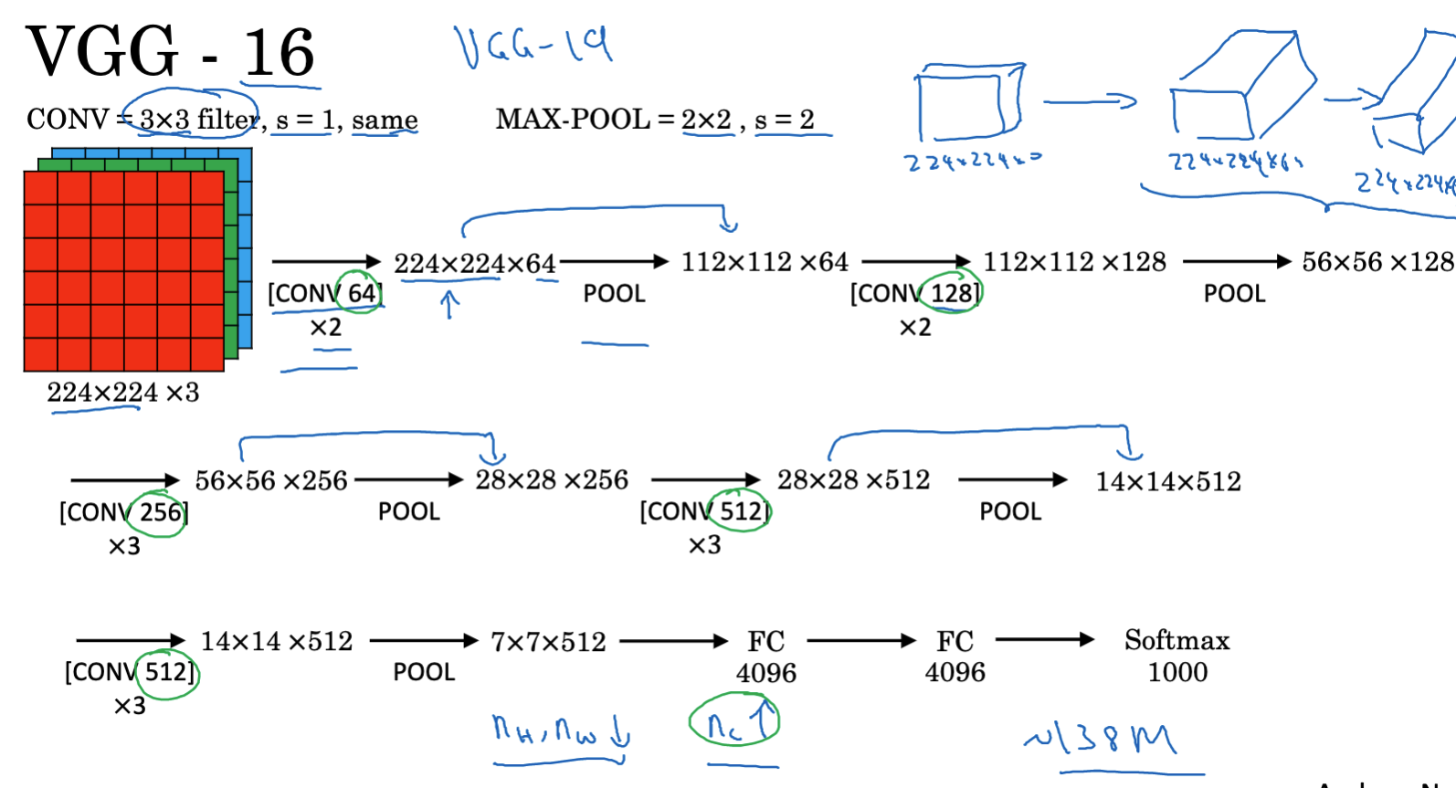
The structure of VGGNet is very simple and easy to understand, making it an important reference for subsequent network designs. These networks have established the position of deep convolutional neural networks in the field of computer vision.

Residual Networks

As models deepen, issues such as gradient vanishing and gradient explosion become more prominent. Residual Networks (ResNet) were introduced to address these challenges, with their key innovation being "skip connections." These connections directly transfer the output from a previous layer to a later layer, bypassing intermediate layers. Consequently, the input to a layer comprises both the output from the previous layer and unaltered information from earlier layers. This enables the network to easily learn identity functions by copying activations from earlier layers to deeper ones.

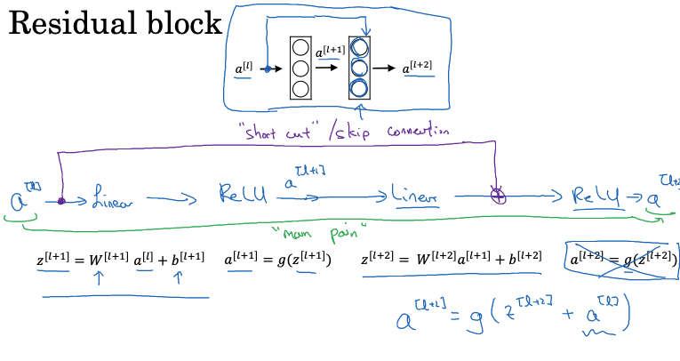
The advantage of this structure is that each layer only needs to learn the residual, or the difference between the input and output. If an identity function needs to be learned, the network only needs to cancel out the residual. The residual structure consists of a main path and a shortcut path (or skip connection). Information can flow directly to deeper layers through the shortcut path, avoiding potential issues in the main path. By stacking numerous residual blocks, a deep network, or ResNet, can be constructed. Adding a shortcut path to a layer and applying ReLU nonlinearity transforms that layer into a residual block.

In deep neural networks, adding more layers does not always improve performance and can even hinder training effectiveness. This is because increasing the number of layers makes it harder to learn identity functions. However, with residual networks, even very deep networks can easily learn a "zero mapping" to transmit information, significantly reducing the training difficulty of deep networks.

During training, L2 regularization reduces the magnitude of weights. If weights and biases are regularized to zero, additional layers can learn the identity function. For skip connections, the dimensions of the early and later layers must match. If they do not, an extra matrix can be used for adjustment. ResNets frequently use 3x3 convolutions to ensure that the input and output dimensions in the skip connections are the same, facilitating addition operations.

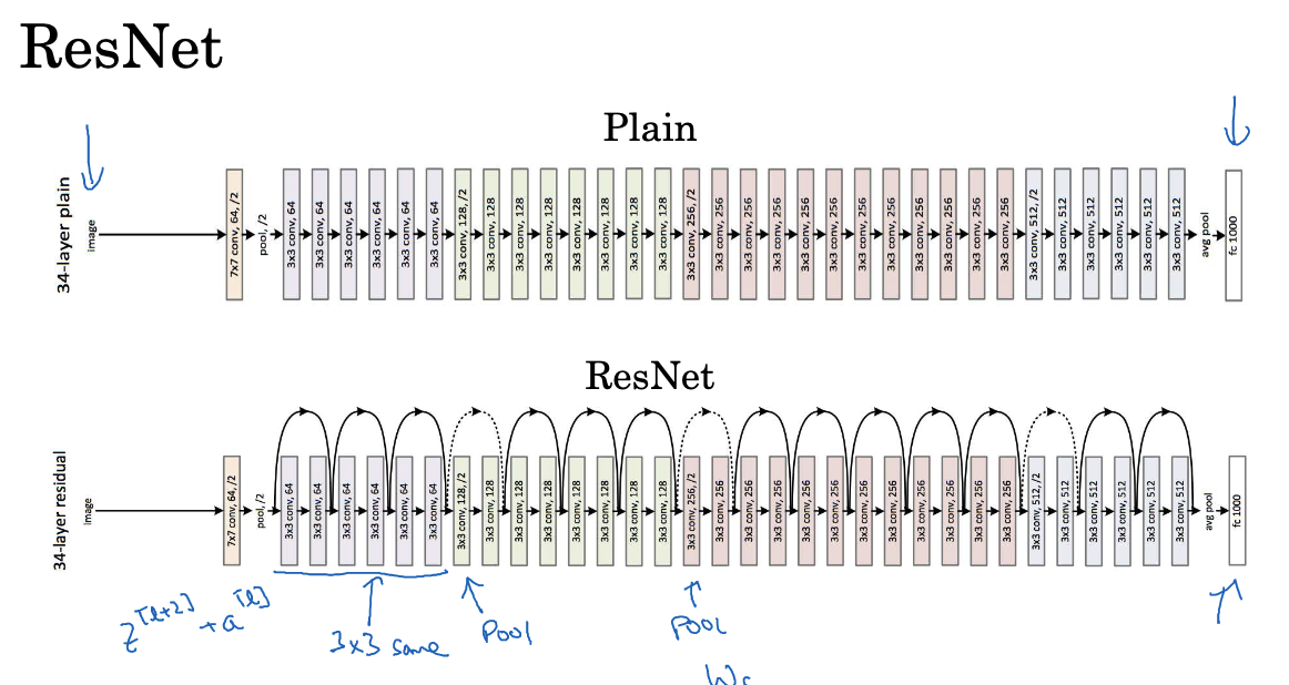
When training neural networks, various optimization algorithms, such as gradient descent, are used. In standard deep neural networks (without residual blocks), training error initially decreases with more layers but then increases, which is undesirable. However, in ResNets, training error continues to decrease even as layers are added. Although it may eventually plateau, ResNets significantly aid in training deep networks effectively.

While some researchers experiment with networks over 1000 layers deep, such networks are rare in practical applications. However, using skip connections or shortcut paths to connect intermediate layer activations to later layers helps mitigate gradient vanishing and explosion issues, enabling the training of deeper neural networks without performance degradation.

The Application of 1x1 Convolution in Networks

When designing network architectures, 1x1 convolution is a very useful concept. For one-dimensional images, 1x1 convolution may not seem particularly useful, as it only multiplies each element of the image by a number. However, for multi-dimensional images, such as 6x6x32 images, 1x1 convolution can perform very meaningful operations.

1x1 convolution processes each position in the image by multiplying the elements at each position by the corresponding filter elements and then applying ReLU nonlinearity to the result. This process can be viewed as a fully connected neural network, where for each position, 32 numbers (from 32 channels at the same position) are input, and the number of filters determines the output.

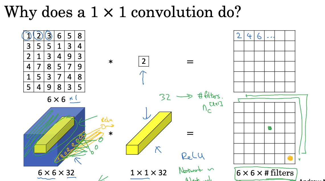
Though 1x1 convolution seems simple, it is crucial for the network in two main ways:

• First, it adjusts the number of channels in the network. For example, if the input is a feature map with 128 channels and we want to convert it to 512 channels for subsequent layers, we can introduce 512 1x1x128 convolution kernels, resulting in 512 output channels.
• Second, it increases nonlinearity. Convolutional layers are essentially linear operations, but by adding 1x1 convolution and applying ReLU or other nonlinear activation functions, we can achieve nonlinear mapping.
  The Inception network uses a large number of 1x1 convolutions to reduce the number of channels and computational load while increasing the network's expressive power.

Inception Networks

The Inception network is a convolutional neural network architecture introduced by Google's research team, including Christian Szegedy, in 2014. This network architecture changed the traditional approach to organizing different types and sizes of convolutional kernels and pooling layers in deep networks.

In traditional convolutional neural networks, designing each layer requires making multiple choices, such as what size of convolutional kernel to use (e.g., 1x1, 3x3, 5x5, etc.) or whether to use a pooling layer. The Inception network proposed a unique solution: why not use all these elements simultaneously? Although this idea makes the network architecture more complex, it also enhances the network's expressive power.

In convolutional neural networks, you can choose the convolutional kernel size you want to use and even decide whether you need convolutional layers or pooling layers. The Inception network chooses to use all these elements simultaneously. For example, a 1x1 convolutional kernel will output a 28x28 result, which is a 28x28x64 output; you can also try a 3x3 convolutional kernel and get a 28x28x128 result; similarly, you can try a 5x5 convolutional kernel and get a 28x28x32 result; additionally, you can use a pooling layer. These different outputs are then stacked along the channel dimension.

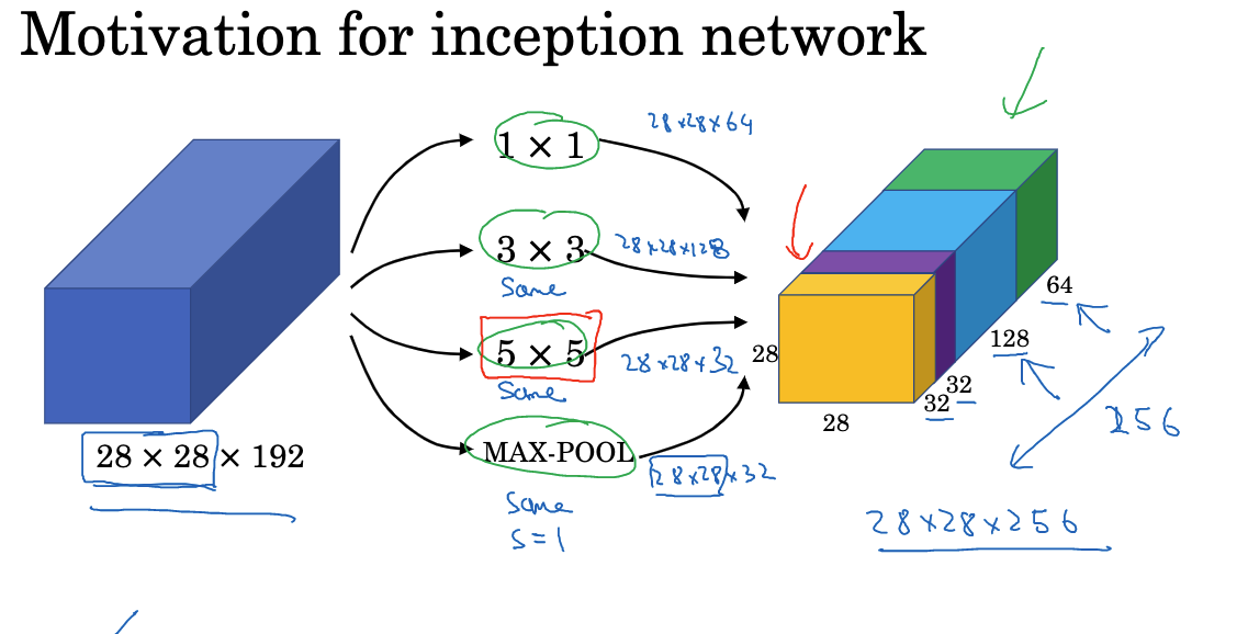
In the Inception network, padding is required to match the output dimensions, which is known as same padding. This ensures that the output dimensions remain 28x28, the same as the input height and width.

Although the Inception module is very powerful, it also increases computational complexity, especially for large-sized convolutional kernels. To address this issue, the Inception network uses "bottleneck layers" to reduce dimensions. Specifically, 1x1 convolutions are used before larger convolution operations to reduce depth (number of channels), thereby reducing computational cost.

The Inception module first extracts features using convolutional kernels of different sizes, such as 1x1, 3x3, and 5x5 convolutional kernels. Then all features are concatenated along the channel dimension. Meanwhile, a parallel branch with max pooling is also introduced. The reason for this design is that convolutional kernels of different sizes are suitable for detecting features of different scales. The 1x1 convolution integrates information across channels, while the 3x3 and 5x5 convolutions detect local features in the spatial dimension. Max pooling retains position invariance. The parallel multi-branch structure in the Inception module allows the network to adapt to different feature information simultaneously. Compared to choosing only one convolutional kernel, this design can extract richer features, thereby improving classification performance. Subsequent versions, Inception V2, V3, and V4, further improved on this by introducing mechanisms such as batch normalization and residual connections to train deeper Inception networks and further widen the network.
The Inception network demonstrates the design approach of enhancing model performance through structural innovation. Its multi-branch parallel structure has inspired and influenced many subsequent networks.

Interestingly, the name "Inception" for this network model was inspired by the movie Inception. In the movie, there is a line that says, "We need to go deeper," which has become a metaphor in the deep learning community, symbolizing the need to build deeper and more complex networks.

Overall, the Inception network, through its innovative module design, computational optimization, and regularization strategies, has not only advanced the development of convolutional neural networks but also set new performance standards in various visual tasks such as image classification and object detection.

Efficient MobileNet

Deploying models on mobile devices requires higher computational efficiency. MobileNet was developed to meet this demand, using techniques such as depthwise separable convolutions to build lightweight and efficient networks.
Depthwise separable convolutions in MobileNet decompose standard convolutions into two steps: first, a depthwise convolution is performed for each channel, and then a 1x1 convolution is performed to integrate information across channels. Compared to standard convolutions that perform spatial and cross-channel operations simultaneously, depthwise separable convolutions greatly reduce computational cost and the number of parameters.

1. Standard Convolution Operation:
   • Suppose the input image size is $n \times n \times n_c$, where $n_c$ is the number of channels. If you use a $f \times f \times n_c$ filter to convolve it, you need to perform $f \times f \times n_c$ multiplications. Then, you need to move the filter to calculate the next value of the output. Assuming the number of filters is $nc'$, the output dimensions will be $n{out} \times n_{out} \times n_c'$.
   • The total computational cost of the standard convolution operation is obtained by multiplying the number of filters, the number of filter parameters, and the number of filter positions.
2. Depthwise Separable Convolution: consists of depthwise convolution and pointwise convolution.
   • Depthwise Convolution: In depthwise convolution, we only use $f \times f$ filters, and the number of filters equals the number of input channels ($nc$). The output size of depthwise convolution is $n{out} \times n_{out} \times n_c$.
   • Pointwise Convolution: Pointwise convolution convolves the output of depthwise convolution ($n{out} \times n{out} \times n_c$) with a $1 \times 1 \times nc$ filter to get the final output $n{out} \times n_{out} \times n_c'$. Note that the number of pointwise convolution filters equals the desired number of output channels ($n_c'$).

Additionally, MobileNet uses inverted residuals and linear bottleneck layers to further improve efficiency. Inverted residuals stabilize network training, while linear bottlenecks reduce memory access costs. Subsequent MobileNet V2 builds on MobileNet, using better-designed inverted residual blocks and more efficient linear bottleneck layers to further improve performance.

The MobileNet series demonstrates that with careful design, it is possible to significantly improve computational efficiency while maintaining performance, allowing complex deep networks to run efficiently on mobile devices. This makes it feasible to widely apply deep learning in the mobile domain.

EfficientNet - Automatic Adjustment Based on Device

Previous work, such as MobileNet V1 and V2, has demonstrated how to construct more computationally efficient models. In contrast to MobileNet's fixed structure, EfficientNet introduces a new method of network scaling that automatically adjusts the network size to fit different hardware platforms. The core idea of EfficientNet is to simultaneously scale the network’s depth, width, and input resolution to achieve optimal performance. Here, network width refers to the number of filters in a layer.

The basic concept behind EfficientNet is to adjust depth, width, and resolution together, rather than individually. By scaling these three dimensions simultaneously, EfficientNet can provide an optimal model for any specific computational constraint. For instance, for a powerful server with abundant computational resources, EfficientNet might select a larger model with high-resolution input and many layers, achieving maximum accuracy. Conversely, for a mobile phone or embedded device with limited computational power, it might select a smaller, shallower model with lower resolution to ensure fast operation.

Another advantage of this method is that it removes the need for manual adjustments of models for different applications. Typically, researchers must conduct extensive experiments and fine-tuning to find the best model for a specific device or application. With EfficientNet, however, you only need to choose an appropriate scaling factor, and the model will automatically adjust to provide optimal performance.

EfficientNet is not just a theoretical idea. The open-source community has already provided multiple implementations for this framework, making it easy for developers to select the right model size for their applications and devices. For those looking to deploy deep learning models on mobile devices, embedded systems, or any environment with limited computational and memory resources, EfficientNet offers a highly attractive solution.

Based on the concept of model scaling, EfficientNet can automatically construct the most efficient model for given hardware conditions. This hardware-driven network design approach allows neural networks to better serve practical applications. EfficientNet’s design philosophy provides a way to quickly build the most suitable model for different application scenarios. This makes it easier to deploy deep learning across various hardware platforms.

Transfer Learning

Transfer learning is a method for building powerful computer vision models, especially when data is scarce. By leveraging network weights and architectures that have been pre-trained on large-scale datasets (such as ImageNet, MSCOCO, PASCAL, etc.), we can transfer these results to new, specific problems.

Key Steps in Transfer Learning:

1. Download network architectures and weights pre-trained on large datasets, such as ImageNet, MSCOCO, PASCAL, etc.
2. Use the downloaded weights and network architectures as the starting point for initializing your own neural network.
3. Adjust the network according to your specific problem, such as modifying the classification layer or adding new output layers.
4. Freeze the earlier layers and only train the parameters of the later layers that are relevant to your specific problem.
5. If the dataset is small, precompute the activation results of the earlier layers and save them to disk to speed up the training process.
6. Depending on the size of the dataset and computational resources, decide how many layers to freeze and how many layers to train; more data allows training more layers.
7. Use transfer learning to train your own network to achieve better performance.

Transfer learning is widely used in computer vision, especially in situations with insufficient data and computational resources. By leveraging pre-trained weights and network architectures, high-performance computer vision applications can be quickly built without starting from scratch. Many deep learning frameworks support methods for freezing layers, setting parameters, and precomputing activation results.

In summary, transfer learning provides a fast and efficient way to develop computer vision applications, achieving good performance with limited resources while avoiding the need to train networks from scratch.

Data Augmentation

Data augmentation is a method used to expand the dataset by applying various transformations (such as rotation, cropping, flipping, etc.) to the original data. These simple yet effective techniques can enhance the model’s generalization ability.

Common Data Augmentation Methods:

1. Mirroring: Flipping the image vertically or horizontally.
2. Random Cropping: Randomly selecting and cropping a portion of the image.
3. Color Jittering: Adding random noise to the RGB channels.
4. Combining Methods: Using multiple methods together to increase data diversity.

For large-scale training sets, multi-threaded loading and processing of image data can improve efficiency. Data augmentation hyperparameters can be adjusted based on specific tasks and requirements. Additionally, using open-source implementations of data augmentation methods can be a good starting point. Overall, data augmentation can improve the robustness and generalization ability of models, enhancing the effectiveness of computer vision applications.

Current Challenges in Computer Vision

Computer vision is an interdisciplinary field that attempts to enable computers to interpret and understand image or video data from the world. Despite significant progress in recent years, the field still faces several major challenges.

1. Data Volume Challenge: Computer vision tasks typically require large amounts of data to train models. Although the scale of existing datasets is continually increasing, for complex problems, the data volume is still insufficient. In contrast, other fields do not require as much data as computer vision. This makes data augmentation particularly useful when training computer vision models.
2. Importance of Manual Design: Computer vision tries to learn very complex functions, so manual design plays a crucial role. When we lack large amounts of labeled data, manual design is key to achieving good results. The field of computer vision still relies heavily on manual design, including feature design, network structure design, and other component designs.
3. Application of Transfer Learning: Transfer learning is a very useful technique in situations with limited data. It allows the use of models pre-trained on large datasets and fine-tuning them for specific tasks. Transfer learning is very effective for solving computer vision problems, especially when we have relatively little data.
4. Importance of Benchmark Datasets: In computer vision research, many people focus on achieving good results on benchmark datasets and winning competitions. Performing well on benchmark datasets helps us understand which algorithms are most effective. However, these methods may not be applicable in real-world products as they often require significant computational resources and runtime.
5. Ensemble Learning and Multi-Crop: Ensemble learning is a technique used to achieve good results in benchmark data testing, but it is often impractical in real-world products. Multi-crop is a form of data augmentation that can be applied to test images. It involves making multiple crops of an image and averaging their results to improve performance.

In summary, deep learning has many unique applications and challenges in computer vision. Manual design still plays a significant role, while techniques such as transfer learning and data augmentation can help achieve better results in situations with limited data. Understanding computer vision architectures and techniques can help us build effective computer vision systems.

Conclusion

In summary, this article introduces some classic cases and core ideas of convolutional neural networks. These cases are valuable references for understanding the design and application of convolutional neural networks. Of course, this article is quite superficial, and for deeper learning, it is recommended to read the original papers.

Reference

1. LeCun Y, Bottou L, Bengio Y, et al. Gradient-based learning applied to document recognition[J]. Proceedings of the IEEE, 1998, 86(11): 2278-2324.
2. Krizhevsky A, Sutskever I, Hinton G E. Imagenet classification with deep convolutional neural networks[J]. Advances in neural information processing systems, 2012, 25.
3. Simonyan K, Zisserman A. Very deep convolutional networks for large-scale image recognition[J]. arXiv preprint arXiv:1409.1556, 2014.
4. He K, Zhang X, Ren S, et al. Deep residual learning for image recognition[C]//Proceedings of the IEEE conference on computer vision and pattern recognition. 2016: 770-778.
5. Lin M, Chen Q, Yan S. Network in network[J]. arXiv preprint arXiv:1312.4400, 2013.
6. Szegedy C, Liu W, Jia Y, et al. Going deeper with convolutions[C]//Proceedings of the IEEE conference on computer vision and pattern recognition. 2015: 1-9.
7. Howard A G, Zhu M, Chen B, et al. Mobilenets: Efficient convolutional neural networks for mobile vision applications[J]. arXiv preprint arXiv:1704.04861, 2017.
8. Sandler M, Howard A, Zhu M, et al. Mobilenetv2: Inverted residuals and linear bottlenecks[C]//Proceedings of the IEEE conference on computer vision and pattern recognition. 2018: 4510-4520.
9. Tan M, Le Q. Efficientnet: Rethinking model scaling for convolutional neural networks[C]//International conference on machine learning. PMLR, 2019: 6105-6114.