Introduction to Deep Learning and Neural Networks

The explosive popularity of ChatGPT and the recent flurry of large-scale model developments have thrust the field of artificial intelligence into the spotlight. As a tech enthusiast keen on exploring various technologies, understanding the principles behind these advancements is a natural inclination. Starting with deep learning is a logical step in delving deeper into AI, especially since I’ve already studied Professor Andrew Ng’s Machine Learning course. Now, through his Deep Learning Specialization, I am furthering my knowledge in this domain. This article aims to demystify deep learning, drawing insights from the first course of the specialization.

1. Neural Networks: An Overview and Fundamental Concepts

Neural networks are algorithmic models that mimic the human brain’s neural network for distributed and parallel information processing. Comprising a vast array of interconnected nodes (or neurons), each neuron processes incoming signals with simple signal processing functions and transmits the outcomes to subsequent neurons. The objective is to minimize the predictive error of the network by continually adjusting the network’s parameters, namely the connection weights between neurons. Below is an illustration showcasing various common neural networks, including standard neural networks, Convolutional Neural Networks (CNN), and Recurrent Neural Networks (RNN).

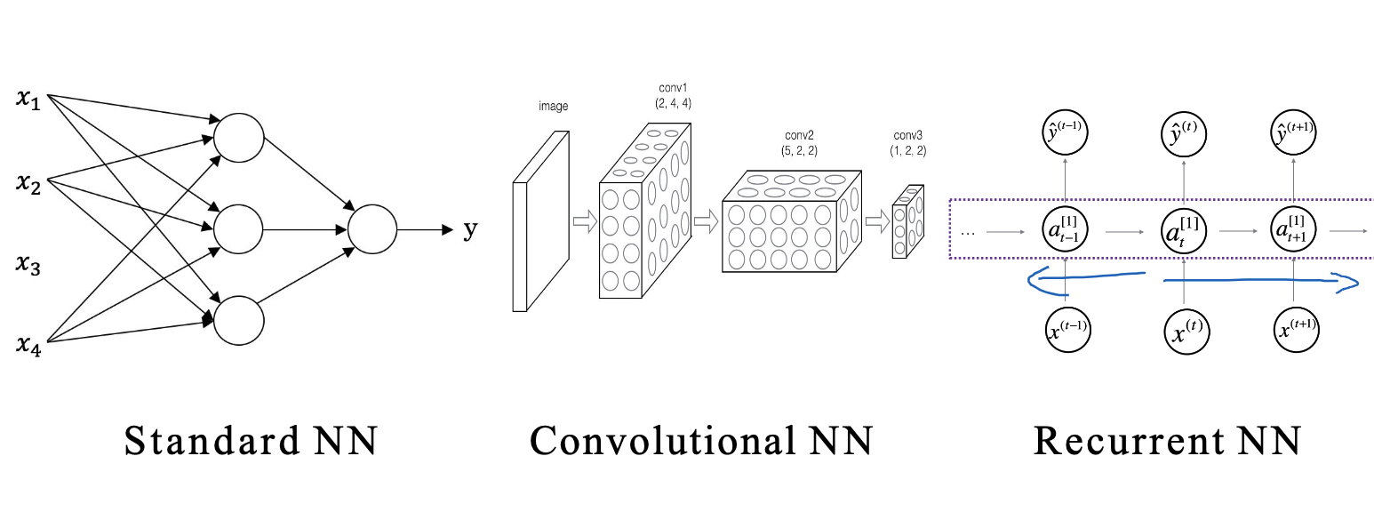Before delving deeper, it’s essential to grasp some key concepts in neural networks.

1.1 Loss Function

The loss function quantifies the disparity between our model’s prediction for a single sample and the actual outcome. In binary classification tasks, the Cross Entropy Loss is frequently utilized. For instance, if our model predicts the likelihood of a sample belonging to a positive class as $\hat{y}$ , and the actual label is $y$ (0 or 1), then the cross-entropy loss is defined as:

$$
L(\hat{y}, y) = -[ylog(\hat{y}) + (1-y)log(1-\hat{y})]
$$

This metric reflects the variance between the actual label and the predicted probability: the loss is near zero when they align closely, but escalates significantly when there is a substantial deviation.

1.2 Cost Function

While the loss function assesses the error for individual samples, the cost function evaluates the aggregate prediction error across the entire training set. It is the mean of all the loss values across samples. For the cross-entropy loss, given $m$ samples, the cost function $J$ is expressed as:

$$
J(w, b) = -\frac{1}{m}\sum_{i=1}^{m}[y^{(i)}log(\hat{y}^{(i)}) + (1-y^{(i)})log(1-\hat{y}^{(i)})]
$$

The aim in neural networks is to identify the optimal values of $w$ and $b$ that minimize the cost function $J(w, b)$ . This optimization is typically achieved through algorithms like gradient descent.

1.3 Gradient Descent

To minimize the cost function, we frequently utilize the optimization technique known as gradient descent. In this process, we calculate the gradient of the cost function concerning each parameter during every iteration, and subsequently update these parameters:

$$
w = w – \alpha \frac{\partial J}{\partial w}
$$

$$
b = b – \alpha \frac{\partial J}{\partial b}
$$

Here, $\alpha$ represents the learning rate, a crucial factor that governs the magnitude of the update steps. The terms $\frac{\partial J}{\partial w}$ and $\frac{\partial J}{\partial b}$ denote the partial derivatives of the cost function $J$ with respect to $w$ and $b$ , indicating the rate of change of $J$ at the current parameters.

Through numerous iterations, we can progressively approach the optimal parameters that minimize the cost function, thereby enhancing our model’s performance.

1.3.1 Variants of Gradient Descent: Batch, Stochastic, and Mini-batch

Gradient descent can be differentiated based on the dataset utilization method into Batch Gradient Descent, Stochastic Gradient Descent, and Mini-batch Gradient Descent.

Batch Gradient Descent: This method involves using the entire dataset for gradient computation and parameter updating in each iteration. Its primary advantage is its accuracy in direction and reduced likelihood of getting stuck in local optima. However, its major drawback is the extensive computational load per iteration when dealing with large datasets, leading to slower processing speeds.
Stochastic Gradient Descent: Here, only a single sample is used for gradient calculation and parameter updating in each iteration. Its main advantage lies in its rapid computation speed and quick convergence, but it also has the drawback of significant fluctuations in update directions due to reliance on single samples, possibly bypassing the global optimum.
Mini-batch Gradient Descent: A blend of the above methods, it utilizes a small batch of samples for gradient calculation and parameter updating in each iteration. This approach balances the benefits of both Batch and Stochastic Gradient Descent, offering reasonable computation speed and gradient direction accuracy. It is the most commonly employed method in practical applications.

1.3.2 Challenges and Solutions in Gradient Descent

Despite being a potent optimization tool, gradient descent presents certain challenges:

Local Optima: There’s a risk of gradient descent converging to local optima instead of the global optimum. To counter this, strategies like random initialization or more sophisticated optimization techniques (e.g., gradient descent with momentum, Adam) are employed.
Vanishing and Exploding Gradients: Deep neural networks might experience very small (vanishing) or very large (exploding) gradients during backpropagation. To address this, strategies like employing non-saturating activation functions (e.g., ReLU) or techniques such as batch normalization and residual structures are used.
Optimal Learning Rate Selection: An excessively high learning rate can prevent gradient descent from converging, while a too-low rate can significantly slow down the process. This issue is tackled using strategies like learning rate decay or adaptive learning rate optimizers, such as Adam.

A profound comprehension of gradient descent enables a better understanding of neural network training, facilitating improved control and optimization of the training process.

1.4 Mathematical Symbols in Neural Networks

Neural networks utilize a variety of mathematical symbols, and it’s essential to familiarize ourselves with some fundamental ones:

$x^{(i)}$: Denotes the feature vector of the $i$th sample.
$y^{(i)}$: Indicates the actual label of the $i$th sample.
$\hat{y}^{(i)}$: Represents the predicted label of the $i$th sample.
$w^{[l]}$: The weight matrix of the $l$th layer.
$b^{[l]}$: The bias vector of the $l$th layer.
$a^{[l]}$: The activation value of the $l$th layer.
$z^{[l]}$: The linear output of the $l$th layer, calculated as $z^{[l]} = w^{[l]}a^{[l-1]}+b^{[l]}$.
$m$: The total number of samples.
$n^{[l]}$: The number of nodes in the $l$th layer.
$n_x$: The number of nodes in the input layer, corresponding to the number of features.
$n_y$: The number of nodes in the output layer, corresponding to the number of label categories.

To simplify, remember these key points:

Square brackets in the upper right signify the $l$ th layer.
Round brackets in the upper right indicate the $i$ th example.
Subscript numbers represent the $n$ th neuron.

Grasping these symbols is like learning the basic language of neural networks, enabling you to understand their operational principles and the mathematical methods for their implementation. Don’t worry if you can’t memorize all these formulas immediately; they will become more familiar as you encounter them throughout your study.

2. Activation Functions

In neural networks, activation functions are crucial. They introduce non-linearity, enabling the network to model complex relationships. This chapter will explore various common activation functions and their unique features.

2.1 Sigmoid Function

The Sigmoid function, one of the earliest used in neural networks, is defined as:

$$
a = \sigma(z) = \frac{1}{1+e^{-z}}
$$

A key feature of this function is that its output ranges between 0 and 1, making it interpretable as a probability. Specifically, as the input z approaches positive infinity, the output a nears 1, and conversely, as z approaches negative infinity, a nears 0. This behavior makes it particularly useful as an output layer activation function in binary classification tasks, providing a probabilistic output.

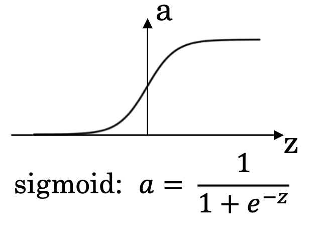
Widely employed in logistic regression, a classification algorithm primarily for binary classification, the Sigmoid function is instrumental in modeling the probability of an event’s occurrence based on input features. The output of logistic regression is this calculated probability.

However, the Sigmoid function has its drawbacks. When inputs have large absolute values, its gradient tends to zero, leading to a vanishing gradient problem that complicates neural network training. Moreover, since its output is not zero-centered, it can slow down the convergence process during training.

2.2 Tanh Function

The Tanh function, an extension of Sigmoid, compresses its input to a range between -1 and 1. Its formula is:

$$
a = \tanh(z) = \frac{e^z-e^{-z}}{e^z+e^{-z}}
$$

With its output centered around zero, the Tanh function often outperforms the Sigmoid function in practical applications.

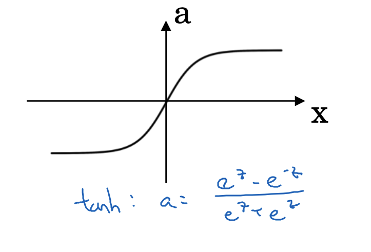
Like the Sigmoid, the Tanh function also faces the issue of vanishing gradients for inputs with large absolute values, where the function’s gradient becomes negligible.

2.3 ReLU Function (Rectified Linear Unit)

The ReLU (Rectified Linear Unit) function is a popular activation function in modern neural networks. It is defined as:

$$
a = \max(0,z)
$$

This function maintains the input value when x is greater than 0, and outputs 0 for x less than 0. The ReLU function’s constant gradient of 1 for positive x values helps in reducing the vanishing gradient problem, a common issue in deep neural networks.

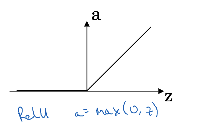
A drawback of ReLU is its complete inactivity for x less than 0, which can lead to ‘neuron death,’ where some neurons fail to activate during training. Additionally, the ReLU function’s output is not zero-centered.

2.4 Leaky ReLU Function

The Leaky ReLU function was developed to address the neuron death issue in the ReLU function. Its formula is:

$$
a = \max(0.01z, z)
$$

Unlike the standard ReLU, Leaky ReLU has a slight slope (0.01) for x less than 0, ensuring that there is a small, yet non-zero gradient. This modification reduces the likelihood of neuron death.

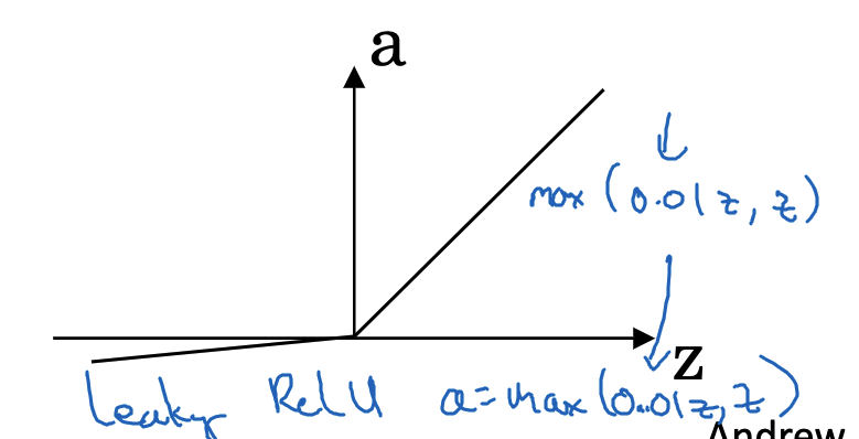
Activation functions are vital in neural networks. Understanding their characteristics and how they fit into different scenarios is key to designing and optimizing neural network models.

3. Forward Propagation

In deep learning, forward propagation is a foundational and critical process, involving the transmission of input data through the neural network to compute the output. This chapter will delve into the specifics of forward propagation, along with some pertinent mathematical details.

3.1 Concept of Forward Propagation

First, let’s define forward propagation. It’s the process in neural networks where each layer’s nodes are computed from the preceding layer’s nodes. Specifically, each layer first calculates a linear combination (weighted sum of inputs) and then applies a non-linear transformation through an activation function.

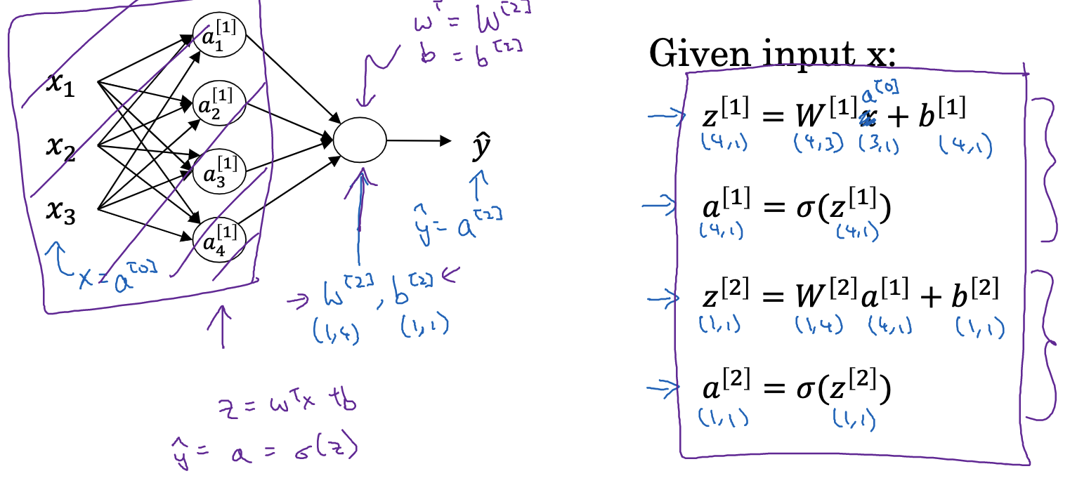
Mathematically, for each node $j$ in layer $l$ , the linear combination is $z_j^{[l]} = \sumi w{ij}^{[l]} a_i^{[l-1]} + bj^{[l]} $. Here,$ w{ij}^{[l]} $is the weight connecting node$ i $in layer$ l-1 $to node$ j $in layer$ l $,$ a_i^{[l-1]} $is the activation value of node$ i $in layer$ l-1 $, and$ b_j^{[l]} $is the bias of node$ j $in layer$ l $. Next, this value is passed through an activation function$ g^{[l]} $, producing the activation value$ a_j^{[l]} = g^{[l]}(z_j^{[l]})$.

3.2 Calculation of the Linear Part

To handle multiple nodes and samples efficiently, we use matrix and vector representations for linear computations. For $m$ samples, inputs are represented as an $n_x \times m$ matrix $X$ , where $n_x$ is the input size (number of nodes in layer 0, the input layer) and $m$ is the sample count.

For layer $l$ , weights are represented by an $n^{[l]} \times n^{[l-1]}$ matrix $W^{[l]}$ , and biases by an $n^{[l]} \times 1$ vector $b^{[l]}$ . Thus, the linear combination for all nodes in layer $l$ is computed as $Z^{[l]} = W^{[l]} A^{[l-1]} + b^{[l]}$ , where $A^{[l-1]}$ represents the activation values of all nodes in layer $l-1$ .

3.3 Calculation of the Non-linear Part

After computing the linear part (Z^{[l]}), we proceed with a nonlinear transformation using an activation function. This function can be any nonlinear function, with common choices being the Sigmoid, tanh, ReLU, and Leaky ReLU functions. The primary role of the activation function is to infuse nonlinearity into the system, allowing the neural network to effectively approximate complex functions. Without the activation function, the network, irrespective of its layers, would equate to a linear model, severely constricting its capacity to express complex relationships.

In the (l^{th}) layer, the computed (Z^{[l]}) is fed into the activation function (g^{[l]}), producing the activation value (A^{[l]} = g^{[l]}(Z^{[l]})). To handle all samples simultaneously, (A^{[l]}) is treated as an (n^{[l]} \times m) matrix, with each column representing a sample and each row a neuron.

As we reach the final layer, the output layer, we acquire the neural network’s output. In binary classification, the Sigmoid function is typically used in the output layer, rendering the output interpretable as the probability of belonging to the positive class. In contrast, for multi-class classification, the softmax function is employed, enabling the interpretation of the output as the probability distribution across different classes.

Upon completing forward propagation, we evaluate the loss function, assessing the deviation between predictions and actual labels. This discrepancy guides the backward propagation phase, wherein network parameters are adjusted to align predictions more closely with the true labels, forming the essence of neural network training.

$$
Z^{[1]} = W^{[1]}x + b^{[1]}
$$

$$
A^{[1]} = g^{[1]}(Z^{[1]})
$$

$$
Z^{[2]} = W^{[2]}A^{[1]} + b^{[2]}
$$

$$
A^{[2]} = g^{[2]}(Z^{[2]})
$$

This narrative encapsulates the forward propagation process. Although rooted in linear algebra and calculus, fundamentally, forward propagation is a deterministic process that transforms input data into output results, solely based on input data and network parameters. Comprehending forward propagation equips us with an understanding of how neural networks process inputs to generate outputs – the ‘first half’ of the neural network’s operation. Subsequently, we’ll explore backward propagation, the ‘second half’ of the network’s functionality.

4. Backpropagation

In the forward propagation process, we explored how a neural network transforms input data into output. However, to enhance its predictive or classification capabilities, we need a metric to gauge the discrepancy between the neural network’s output and the desired output. This metric is known as the loss function. Once the loss function is established, our objective is to discover a method to minimize this loss. This method is termed backpropagation, involving the computation of the loss function’s gradient and subsequently updating the neural network’s parameters based on this gradient. This chapter delves into the principles and processes of backpropagation in detail.

4.1 Calculating the Gradient

Previously, we introduced the cost function. Our aim is to find a method to minimize this function. As the cost function is dependent on the neural network’s parameters, altering these parameters can modify the cost function’s value. The fundamental principle of gradient descent is as follows: we compute the partial derivative, or the gradient, of the cost function with respect to each parameter and then update the parameters in the direction opposite to the gradient.

Specifically, for the weights $W^{[l]}$ and biases $b^{[l]}$ of the $l^{th}$ layer, it is necessary to calculate their respective partial derivatives $\frac{\partial J}{\partial W^{[l]}}$ and $\frac{\partial J}{\partial b^{[l]}}$ . The complexity of neural network computations necessitates the use of the chain rule for these derivative calculations. This process is referred to as backward propagation, as it begins from the final layer and progresses backward through the layers, transmitting the gradient.

To simplify the calculation, we first determine an intermediate variable $dZ^{[l]} = \frac{\partial J}{\partial Z^{[l]}}$ . This allows us to express

$$
\frac{\partial J}{\partial W^{[l]}} = \frac{1}{m} dZ^{[l]} A^{[l-1]T}
$$

$$
\frac{\partial J}{\partial b^{[l]}} = \frac{\partial J}{\partial b^{[l]}} = \frac{1}{m} np.sum(dZ^{[l]}, axis=1, keepdims=True)$$ where $np.sum$ denotes matrix summation, axis=1 indicates summation along the row direction, and keepdims=True ensures the original dimensions are maintained.

The value of $dZ^{[l]}$ is obtained through the chain rule:
$dZ^{[l]} = dA^{[l]} _ g’^{[l]}(Z^{[l]})$ where $$ represents element-wise multiplication, and $g’^{[l]}$ is the derivative of the activation function.
$dA^{[l]} = \frac{\partial J}{\partial A^{[l]}} = dZ^{[l+1]} W^{[l+1]T}$

Through this method, we can sequentially transmit the gradient backward through the layers, culminating at the first layer. This entire process constitutes backpropagation.

4.2 Parameter Updating

After obtaining the gradient, we proceed with updating the parameters. Specifically, the weights and biases of the $l^{th}$ layer are updated according to the following formulas:

$$
W^{[l]} = W^{[l]} – \alpha \frac{\partial J}{\partial W^{[l]}}
$$

$$
b^{[l]} = b^{[l]} – \alpha \frac{\partial J}{\partial b^{[l]}}
$$

Here, $\alpha$ represents the learning rate, a hyperparameter that dictates the step size in updating parameters. The terms $\frac{\partial J}{\partial W^{[l]}}$ and $\frac{\partial J}{\partial b^{[l]}}$ are the gradients calculated during backpropagation. Through this process, we incrementally reduce the loss function’s value, thereby enhancing the neural network’s performance.

4.3 Overview of Backpropagation Formulas

$$
dZ^{[L]} = A^{[L]} – Y
$$

$$
dW^{[L]} = \frac{1}{m}dZ^{[L]}A^{{[L-1]}^T}
$$

$$
db^{[L]} = \frac{1}{m}np.sum(dZ^{[L]}, axis=1, keepdims=True)
$$

$$
dZ^{[L-1]} = dW^{{[L]}^T}dZ^{[L]} * g’^{[L]}(Z^{[L-1]})
$$

$$
…
$$

$$
dZ^{[1]} = dW^{{[L]}^{T}}dZ^{[2]} * g’^{[1]}(Z^{[1]})
$$

$$
dW^{[1]} = \frac{1}{m}dZ^{[1]}A^{{[1]}^T}
$$

$$
db^{[1]} = \frac{1}{m}np.sum(dZ^{[1]}, axis=1, keepdims=True)
$$

The aforementioned outlines the backpropagation process. It is primarily concerned with calculating gradients and updating parameters. While it involves aspects of calculus and linear algebra, fundamentally, understanding gradient descent and the chain rule is key to grasping backpropagation. Comprehending backpropagation enables us to understand how neural networks adjust their parameters in response to the differences between input and output, essentially unveiling the "latter half" of neural network functionality. In the next chapter, we will implement a simple neural network using Python, providing a more in-depth understanding of both forward and backward propagation.

5. Implementing a Neural Network in Python

Having grasped the fundamental principles of neural networks, this chapter will focus on implementing a basic neural network demo using Python.

5.1 Constructing a Neural Network

The process encompasses initializing parameters, forward and backward propagation, updating parameters, optimization functions, and defining the model. Initially, parameters need to be initialized. It is important to note that W should be initialized randomly, not with zeros, to prevent the first layer of neurons from producing identical zero outputs.

def initialize_parameters(n_x, n_h, n_y):
    np.random.seed(1)

    W1 = np.random.randn(n_h, n_x) * 0.01
    b1 = np.zeros((n_h, 1))
    W2 = np.random.randn(n_y, n_h) * 0.01
    b2 = np.zeros((n_y, 1))

    parameters = {"W1": W1,
                  "b1": b1,
                  "W2": W2,
                  "b2": b2}

    return parameters

Subsequently, functions for forward and backward propagation need to be defined.

# Define the sigmoid function
def sigmoid(Z):
    A = 1 / (1 + np.exp(-Z))
    cache = Z
    return A, cache

# Forward propagation function
def forward_propagation(X, parameters):
    W1 = parameters["W1"]
    b1 = parameters["b1"]
    W2 = parameters["W2"]
    b2 = parameters["b2"]

    Z1 = np.dot(W1, X) + b1
    A1 = np.tanh(Z1)
    Z2 = np.dot(W2, A1) + b2
    A2, cache = sigmoid(Z2)

    cache = {"Z1": Z1,
             "A1": A1,
             "Z2": Z2,
             "A2": A2}

    return A2, cache

# Compute the Cost Function
def compute_cost(A2, Y):
    m = Y.shape[1]

    logprobs = np.multiply(np.log(A2), Y) + np.multiply((1 - Y), np.log(1 - A2))
    cost = - np.sum(logprobs) / m

    cost = np.squeeze(cost)

    return cost

# Backward propagation function
def backward_propagation(parameters, cache, X, Y):
    m = X.shape[1]

    W1 = parameters["W1"]
    W2 = parameters["W2"]
    A1 = cache["A1"]
    A2 = cache["A2"]

    dZ2 = A2 - Y
    dW2 = (1 / m) * np.dot(dZ2, A1.T)
    db2 = (1 / m) * np.sum(dZ2, axis=1, keepdims=True)
    dZ1 = np.multiply(np.dot(W2.T, dZ2), 1 - np.power(A1, 2))
    dW1 = (1 / m) * np.dot(dZ1, X.T)
    db1 = (1 / m) * np.sum(dZ1, axis=1, keepdims=True)

    grads = {"dW1": dW1,
             "db1": db1,
             "dW2": dW2,
             "db2": db2}

    return grads

# Function for updating parameters
def update_parameters(parameters, grads, learning_rate=1.2):
    W1 = parameters["W1"]
    b1 = parameters["b1"]
    W2 = parameters["W2"]
    b2 = parameters["b2"]

    dW1 = grads["dW1"]
    db1 = grads["db1"]
    dW2 = grads["dW2"]
    db2 = grads["db2"]

    W1 = W1 - learning_rate * dW1
    b1 = b1 - learning_rate * db1
    W2 = W2 - learning_rate * dW2
    b2 = b2 - learning_rate * db2

    parameters = {"W1": W1,
                  "b1": b1,
                  "W2": W2,
                  "b2": b2}

    return parameters

Next, an optimization function is needed for multiple training iterations, each consisting of one forward propagation, loss calculation, one backward propagation, and parameter updating.

def optimize(parameters, X, Y, num_iterations=10000, learning_rate=1.2, print_cost=False):
    costs = []

    for i in range(0, num_iterations):
        A2, cache = forward_propagation(X, parameters)
        cost = compute_cost(A2, Y)
        grads = backward_propagation(parameters, cache, X, Y)
        parameters = update_parameters(parameters, grads, learning_rate)

        if print_cost and i % 1000 == 0:
            print ("Cost after iteration %i: %f" %(i, cost))
            costs.append(cost)

    return parameters, costs

Lastly, a model function is required to integrate all these steps, including parameter initialization and multiple training iterations to acquire the trained parameters.

def model(X_train, Y_train, X_test, Y_test, n_h=4, num_iterations=10000, learning_rate=1.2, print_cost=True):
    np.random.seed(3)

    n_x = X_train.shape[0]
    n_y = Y_train.shape[0]

    parameters = initialize_parameters(n_x, n_h, n_y)
    parameters, costs = optimize(parameters, X_train, Y_train, num_iterations, learning_rate, print_cost)

    return parameters, costs

Through these steps, a simple three-layer neural network model is developed. While elementary, it encapsulates the core concepts of neural networks: forward propagation, loss computation, backward propagation, and parameter updating. This example aims to facilitate a better understanding of the principles and operating mechanisms of neural networks.

Indeed, real-world deep learning tasks are much more complex, potentially involving intricate network structures, advanced loss functions, regularization, optimizers, batch normalization, and more. However, understanding this basic example is a crucial first step in the journey of deep learning.